GridDB technical reference
Revision: 1818
Table of Contents
- 1 Introduction
- 2 What is GridDB?
- 3 Structure of GridDB
- 4 GridDB functions
- 4.1 Resource management
- 4.2 User management
- 4.3 Data management function
- 4.3.1 Container (table) data type
- 4.3.2 GEOMETRY-type (Spatial-type)
- 4.3.3 Container (table) ROWKEY
- 4.3.4 Container (table) index
- 4.3.5 Timeseries container (timeseries table)
- 4.3.6 Selection and interpolation of a timeseries container (timeseries table)
- 4.3.7 Affinity function
- 4.3.8 Table partitioning (GridDB AE/VE)
- 4.3.9 Container placement information
- 4.3.10 Block data compression
- 4.3.11 Deallocation of unused data blocks
- 4.4 Transaction processing
- 4.5 Trigger function
- 4.6 Failure process function
- 4.7 Data access
- 4.8 Operating function
- 5 Parameters
- 6 Terminology
- 7 System limiting values
1 Introduction
1.1 Aim & configuration of this manual
This manual explains the GridDB architecture and functions provided.
This manual is targeted at administrators who are in-charge of the operational management of GridDB and designers and developers who perform system design and development using GridDB.
The manual is composed as follows.
-
What is GridDB?
- Describes the features and application examples of GridDB.
-
Architecture of GridDB
- Describes the data model and cluster operating structure in GridDB.
-
Functions provided by GridDB
- Describes the data management functions, functions specific to the data model and operating functions provided by GridDB.
-
Parameters
- Describes the parameters to control the operations in GridDB.
2 What is GridDB?
GridDB is a distributed NoSQL database to manage a group of data (known as a row) that is made up of a key and multiple values. Besides having a composition of an in-memory database that arranges all the data in the memory, it can also adopt a hybrid composition combining the use of a disk (including SSD as well) and a memory. By employing a hybrid composition, it can also be used in small scale, small memory systems.
In addition to the 3 Vs (volume, variety, velocity) required in big data solutions, data reliability/availability is also assured in GridDB. Using the autonomous node monitoring and load balancing functions, laborsaving can also be realized in cluster applications.
2.1 Features of GridDB
2.1.1 Big data (volume)
As the scale of a system expands, the data volume handled increases and thus the system needs to be expanded so as to quickly process the big data.
System expansion can be broadly divided into 2 approaches - scale-up (vertical scalability) and scale-out (horizontal scalability).
-
What is scale-up?
This approach reinforces the system by adding memory to the operating machines, using SSD for the disks, adding processors, and so on. Generally, there is a need to stop the nodes once during scale-up operation as it is not a cluster application using multiple machines even though each individual processing time is shortened and the system processing speed is increased. When a failure occurs, failure recovery is also time-consuming.
-
What is scale-out?
This approach increases the number of nodes constituting a system to improve the processing capability. Generally, there is no need to completely stop service when a failure occurs and during maintenance as multiple nodes are linked and operating together. However, the application management time and effort increases as the number of nodes increases. This architecture is suitable for performing highly parallel processing.
In GridDB, in addition to the scale-up approach to increase the number of operating nodes and reinforce the system, new nodes can be added to expand the system with a scale-out approach to incorporate nodes into an operating cluster.
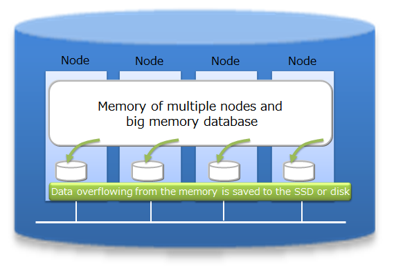
As an in-memory processing database, GridDB can handle a large volume of data with its scale-out model. In GridDB, data is distributed throughout the nodes inside a cluster that is composed of multiple nodes. Therefore, a large-scale memory database can be provided as the memories of multiple nodes can be used as a single, large memory space.
In addition, since data management of a hybrid composition that combines the use of disk with memory is also possible, data exceeding the memory size can be retained and accessed even when operating with a standalone node. A large capacity that is not limited by the memory size can also be realized.
Combined use of in-memory/disk
System expansion can be carried out online with a scale-out approach. As a result, a system in operation can be supported without having to stop it as it will support the increasing volume of data as the system grows.
In the scale-out approach, data is arranged in an appropriate manner according to the load of the system in the nodes built into the system. As GridDB will optimize the load balance, the application administrator does not need to worry about the data arrangement. Operation is also easy because a structure to automate such operations has been built into the system.
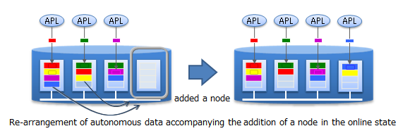
Scale-out model
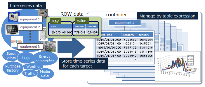
2.1.2 Various data types (variety)
GridDB data adopts a Key-Container data model that is expanded from Key-Value. Data is stored in a device equivalent to a RDB table known as a container. (A container can be considered a RDB table for easier understanding.)
When accessing data in GridDB, the model allows data to be short-listed with a key thanks to its Key-Value database structure, allowing processing to be carried out at the highest speed. A design that prepares a container serving as a key is required to support the entity under management.
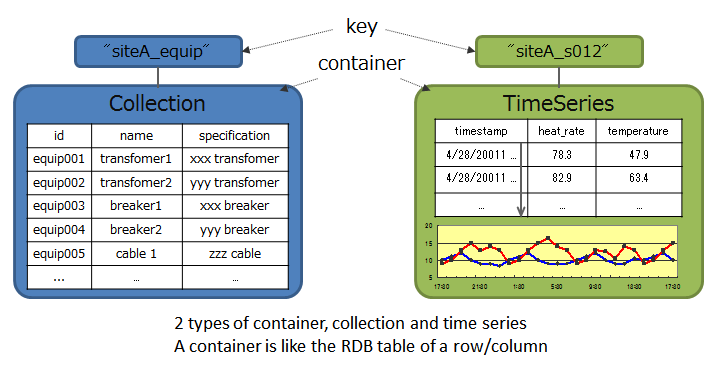
Data model
Besides being suitable for handling a large volume of time series data (TimeSeries container) that is generated by a sensor or the like and other values paired with the time of occurrence, space data such as position information, etc. can also be registered and space specific operations (space intersection) can also be carried out in a container. A variety of data can be handled as the system supports non-standard data such as array data, BLOB and other data as well.
A unique compression function and a function to release data that has expired and so on are provided in a TimeSeries container, making it suitable for the management of data which is generated in large volumes.
2.1.3 High-speed processing (velocity)
A variety of architectural features is embedded in GridDB to achieve high-speed processing.
2.1.3.1 Processing is carried out in the memory space as much as possible
In the case of an operating system with an in-memory in which all the data is arranged, there is no real need to be concerned about the access overhead in the disk. However, in order to process a volume of data so large that it cannot be saved in the memory, there is a need to localize the data accessed by the application and to reduce access to the data arranged in the disk as much as possible.
In order to localize data access in GridDB, a function is provided to arrange related data in the same block as far as possible. Since data in the data block can be consolidated according to the hints provided in the data, memory mishit is reduced during data access, thereby increasing the processing speed for data access. By setting hints for memory consolidation according to the access frequency and access pattern in the application, limited memory space can be used effectively for operation. (Affinity function)
2.1.3.2 Reduces the overhead
In order to reduce events that cause delay in the database execution by as much as possible e.g. a lock or latch event when accessing the database in parallel, exclusive memory and DB files are assigned to each CPU core and thread, so as to eliminate time spent waiting for exclusion and synchronization processing to be carried out.
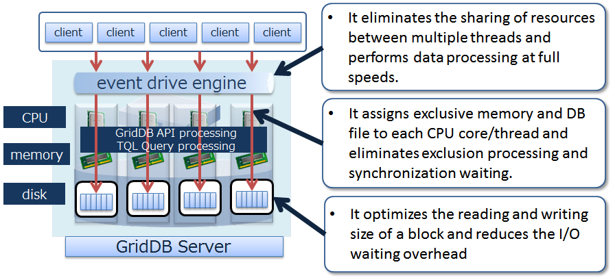
Architecture
In addition, direct access between the client and node is possible in GridDB by caching the data arrangement when accessing the database for the first time on the client library end. Since direct access to the target data is possible without going through the master node to manage the operating status of the cluster and data arrangement, access to the master node can be centralized to reduce communication cost substantially.
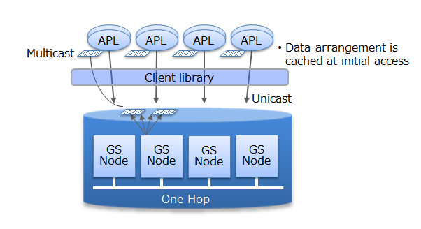
Access from a client
2.1.3.3 Processing in parallel
High-speed processing is realized through parallel processing e.g. by dividing a request into processing units capable of parallel processing in the drive engine and executing the process using a thread in the node and between nodes, as well as dispersing a single large data into multiple nodes (partitioning) for processing to be carried out in parallel between nodes.
2.1.4 Reliability/availability
Duplicate data (hereinafter referred to replicas) are created in the cluster and processing can be continued by using these replicas even when a failure occurs in any of the nodes constituting a cluster. Special operating procedures are not necessary as the system will also automatically perform re-arrangement of the data after a node failure occurs (autonomous data arrangement). Data arranged in a failed node is restored from a replica and then the data is re-arranged so that the set number of replicas is reached automatically.
Duplex, triplex or multiplex replica can be set according to the availability requirements.
Each node performs persistence of the data update information using a disk, and all registered and updated data up to that point in time can be restored without being lost even if a failure occurs in the entire cluster system.
In addition, since the client also possesses cache information on the data arrangement and management, upon detecting a node failure, it will automatically perform a failover and data access can be continued using a replica.
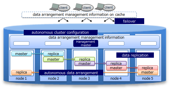
High availability
2.2 GridDB Editions
There are currently three distinct versions of GridDB available.
- GridDB Standard Edition
- GridDB Advanced Edition
- GridDB Vector Edition
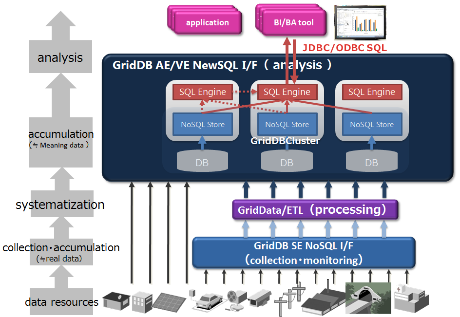
GridDB Advanced Edition (hereinafter referred to as AE) adds SQL processing engine on top of the high performance offered in GridDB Standard Edition (hereinafter referred to as SE). Containers can be considered as tables and operated.
GridDB Vector Edition (hereinafter referred to as VE) is a product added to GridDB AE for high speed matching of high dimensional vector data used in image recognition, machine learning in big data analysis and large scale media analysis.
All products features are described in Features of GridDB.
GridDB AE has 2 additional features as shown below.
-
NewSQL interfaces
- In addition to being SQL 92 compliant, GridDB AE supports ODBC (C language interface) and JDBC (Java interface) application interfaces.
- By using ODBC/JDBC, direct access to the database from BI (Business Intelligence) or ETL (Extract Transfer Load) tool becomes possible.
-
Table partitioning function
- Partitioning function for high speed access to a huge table.
- Since data is divided into multiple parts and distributed to multiple nodes, it is possible to parallelize data search and extraction from the table, thus realizing faster data access.
GridDB VE has 2 additional features as shown below:
-
Ultra-high-speed vector processing
- Realize ultra-high-speed vector processing by expressing data in high-dimension vectors and pre-indexing similar vector groups.
-
Pattern analyze by extended SQL
- Arbitrary pattern analysis can be performed freely with extended SQL that incorporates pattern recognition function.
GridDB editions
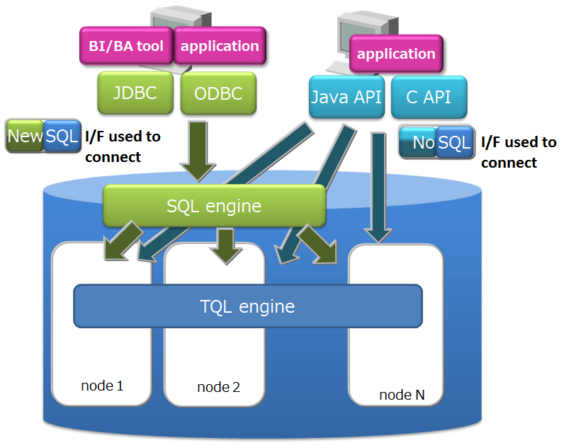
The features of each interface are as follows.
-
NoSQL interface (NoSQL I/F)
- Client APIs (C, Java) of NoSQL I/F focus on batch processing of big data at high speed.
- It is used for data collection, high-speed access of key value data, simple aggregate calculation using TQL, etc.
-
NewSQL interface (NewSQL I/F) (GridDB AE/VE only)
- ODBC/JDBC of NewSQL I/F focus on cooperation with existing applications and development productivity using SQL.
- It is used to classify and analyze data collected using BI tools, etc.
When using GridDB AE/VE, both NoSQL I/F and NewSQL I/F can be used depending on the use case.
Use case
Since GridDB SE and AE share the same data structure, GridDB SE data can be used in GridDB AE.
The database and NoSQL/NewSQL inteface of GridDB have compatibility among the same major version (for the minor version up). The notation of version is as follows.
-
The version of GridDB is represented as "X.Y[.Z]", and each symbol represents the following.
- Major version (X) ・・・ It is changed for significant enhancements.
- Minor version (Y) ・・・ It is changed for expanding or adding functions.
- Revision (X) ・・・ It is changed for such as bug fixes.
When replacing GridDB SE with GridDB AE/VE or when using both NoSQL I/F and NewSQL I/F in GridDB AE/VE, it is necessary to understand the following specification in advance. It is unnecessary when using only GridDB SE.
- Containers created with NoSQL I/F can be accessed as tables in NewSQL I/F. And tables created with NewSQL I/F can be accessed as containers in NoSQL I/F.
- The names of tables and containers must be unique.
- In GridDB SE/AE/VE, the data structure of the database and user management information is common.
3 Structure of GridDB
The operating structure and data model of a GridDB cluster is described.
3.1 Composition of a cluster
GridDB is operated by clusters which are composed of multiple nodes. To access the database from an application system, the nodes have to be started up and the cluster has to be constituted (cluster service is executed).
A cluster is formed and cluster service is started when a number of nodes specified by the user joins the cluster. Cluster service will not be started and access from the application will not be possible until all nodes constituting a cluster have joined the cluster.
A cluster needs to be composed even when operating with 1 node only. In this case, the number of nodes constituting a cluster is 1. A composition that operates a single node is known as a single composition.
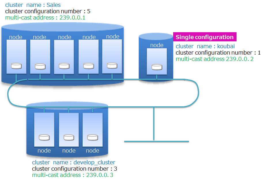
Cluster name and number of nodes constituting a cluster
Cluster names are used to separate multiple clusters so that the correct clusters (using the intended nodes) can be composed using multiple GridDB nodes on a network. Multiple GridDB clusters can be composed in the same network. A cluster is composed of nodes with the same cluster name, number of nodes constituting a cluster, multi-cast address setting. When composing a cluster, the parameters need to be specified as well in addition to setting the cluster name in the cluster definition file which is a definition file saved for each node constituting a cluster.
The method of constituting a cluster using multicast is called multicast method. See Cluster configuration methods for details.
The operation of a cluster composition is shown below.
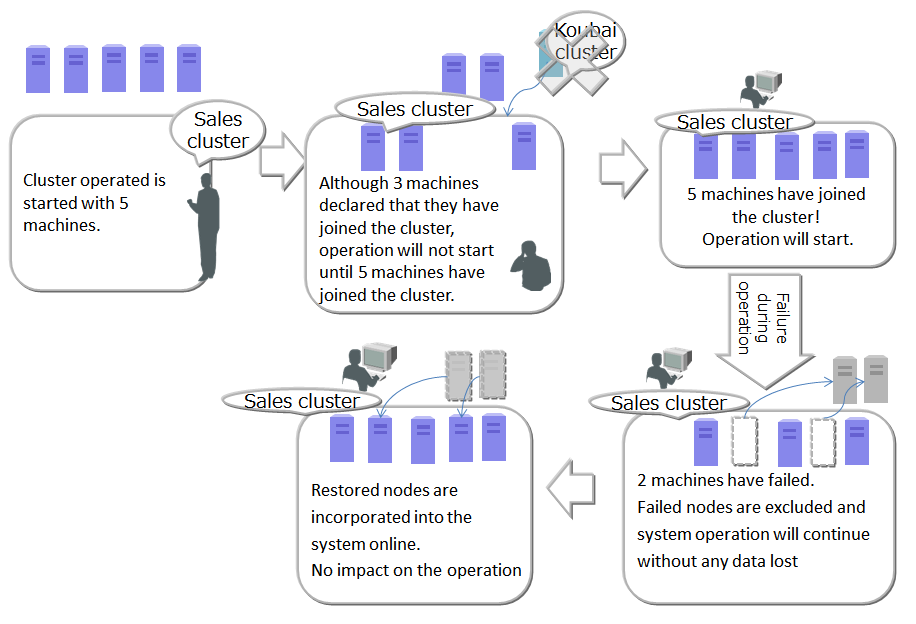
Operation of a cluster composition
To start up a node and compose a cluster, the operation commands gs_startnode/gs_joincluster command or gs_sh are used. In addition, there is a service control function to start up the nodes at the same time as the OS and to compose the cluster.
To compose a cluster, the number of nodes joining a cluster (number of nodes constituting a cluster) and the cluster name must be the same for all the nodes joining the cluster.
Even if a node fails and is separated from the cluster after operation in the cluster started, cluster service will continue so long as the majority of the number of nodes is joining the cluster.
Since cluster operation will continue as long as the majority of the number of nodes is in operation, when a node is separated online due to maintenance and other work during cluster operation, it can be incorporated after the maintenance work ends. Furthermore, nodes can be added online to reinforce the system.
3.1.1 Status of node
There are 2 GridDB status, nodeStatus and clusterStatus that can be checked with a gs_stat command. The status of a node is determined by these 2 statuses.
nodeStatus indicates the operating status of the node while clusterStatus indicates the role of each node in the constituted cluster. The status of the entire cluster is determined by the status of these multiple nodes belonging to the cluster.
-
Transition in the node status
The node status may be one of the following statuses shown in the diagram below.
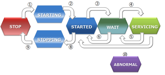
Node status
- [STOP]: State in which the GridDB server has not been started in the node.
- [STARTING]: State in which the GridDB server is starting in the node. Depending on the previous operating state, start-up processes such as recovery processing of the database are carried out. The only possible access from a client is checking the status of the system with a gs_stat command or gs_sh command. Access from the application is not possible.
- [STARTED]: State in which the GridDB server has been started in the node. However, continued access from the application is not possible as the node has not joined the cluster. To obtain the cluster composition, a command is issued to join a cluster with the gs_joincluster or gs_sh cluster operating command.
- [WAIT]: State in which the system is waiting for the cluster composition. Nodes have been informed to join a cluster but the number of nodes constituting a cluster is insufficient, so the system is waiting for the number of nodes constituting a cluster to be reached. It also indicates the node status when the number of nodes constituting a cluster drops below the majority and the cluster service is stopped.
- [SERVICING]: State in which a cluster has been constituted and access from the application is possible. However, access may be delayed if synchronization between the clusters of the partition occurs due to a re-start after a failure when the node is stopped or the like.
- [STOPPING]: Intermediate state in which a node has been instructed to stop but has not stopped yet.
- [ABNORMAL]: SERVICING state or state in which an error is detected by the node in the middle of the state transition. A node in the ABNORMAL state will be automatically separated from the cluster. After obtaining the operating information of the system, the system needs to be stopped by force and then re-started. By re-starting the system, recovery processing will be automatically carried out.
-
Description of state transition
A description of events that serve as an opportunity to change the status of a node.
State transition State transition event Description 1 Command execution Node start-up using gs_startnode command, gs_sh, service start-up 2 System Automatic transition at the end of recovery processing or loading of database files 3 Command execution Cluster participation using gs_joincluster/gs_appendcluster command, gs_sh, service start-up 4 System State changes when the required number of component nodes join a cluster 5 System When other nodes that make up a cluster are detached from the service due to a failure, etc., and the number of nodes constituting a cluster drops below half of the value set. 6 Command execution Detaches a node from a cluster using a gs_leavecluster command or gs_sh 7 Command execution Detaches a node from a cluster using a gs_leavecluster/gs_stopcluster command or gs-sh 8 Command execution Stops a node using gs_stopnode command, gs_sh, service stop 9 System Stops the server process once the final processing ends 10 System Detached state due to a system failure. In this state, the node needs to be stopped by force once. -
Node status and nodeStatus, clusterStatus
By using a gs_stat command, the detailed operating information of the node can be checked with text in the json format. The relationship between the clusterStatus and the nodeStatus which is a json parameter to indicate the gs_stat is shown below.
Status /cluster/nodeStatus /cluster/clusterStatus STARTING INACTIVE SUB_CLUSTER STARTED INACTIVE SUB_CLUSTER WAIT ACTIVATING or DEACTIVATING SUB_CLUSTER SERVICING ACTIVE MASTER or FOLLOWER STOPPING NORMAL_SHUTDOWN SUB_CLUSTER ABNORMAL ABNORMAL SUB_CLUSTER The status of the node can be checked with gs_sh or gs_admin.
3.1.2 Status of cluster
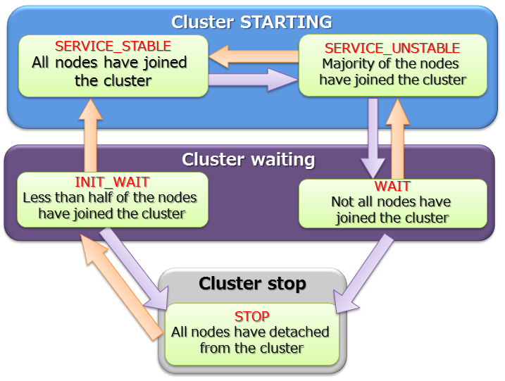
The cluster operating status is determined by the state of each node, and the status may be one of 3 states - IN OPERATION/INTERRUPTED/STOPPED.
Cluster service starts when all the nodes that make up a cluster (number of nodes constituting a cluster) specified by the user during initial system construction have joined the cluster.
During initial cluster construction, the state in which the cluster is waiting to be composed when all the nodes that make up the cluster have not been incorporated into the cluster is known as [INIT_WAIT]. When the number of nodes constituting a cluster has joined the cluster, the state will automatically change to the operating state.
There are 2 operating states. These are [STABLE] and [UNSTABLE].
-
[STABLE] state
- State in which a cluster has been formed by the number of nodes specified in the number of nodes constituting a cluster and service can be provided in a stable manner.
-
[UNSTABLE] state
- State in which the number of nodes constituting a cluster has not been fulfilled.
- Cluster service will continue for as long as a majority of the number of nodes constituting a cluster is in operation.
A cluster can be operated in an [UNSTABLE] state as long as a majority of the nodes are in operation even if they are detached from a cluster due to maintenance and other reasons.
Cluster service is interrupted automatically in order to prevent a split brain from occurring when the number of nodes making up a cluster falls below the majority of the number of nodes constituting a cluster. The state in which cluster service has been interrupted is known as [WAIT] state.
-
What is split brain?
A split brain is an action where multiple cluster systems performing the same process provide simultaneous service when a system is divided due to a hardware or network failure in a tightly-coupled system that works like a single server interconnecting multiple nodes. If the operation is continued in this state, data saved as replicas in multiple clusters will be treated as master data, resulting in data consistency being lost.
To restart cluster service from the [WAIT] state, new nodes are added to a cluster and nodes with errors are restored. The state will become [STABLE] once the number of nodes constituting a cluster has joined the cluster again.
When the number of clusters constituting a cluster falls below half due to a failure in a node constituting the cluster and the cluster operation is disrupted, new nodes are added to a cluster and nodes with errors are restored. Cluster service is automatically restarted once a majority of the nodes has joined the cluster.
Cluster status
A STABLE state is a state in which the value of the json parameter shown in gs_stat, /cluster/activeCount, is equal to the value of /cluster/designatedCount.
%gs_stat -u admin/admin -s
{
    "checkpoint": {
        "archiveLog": 0,
          :
          :
    },
    "cluster": {
        "activeCount":4,                     // Nodes in operation within the cluster
        "clusterName": "test-cluster",
        "clusterStatus": "MASTER",
        "designatedCount": 4,                // Number of nodes constituting a cluster
        "loadBalancer": "ACTIVE",
        "master": {
            "address": "192.168.0.1",
            "port": 10040
        },
        "nodeList": [                        // Node list constituting a cluster
            {
                "address": "192.168.0.1",
                "port": 10040
            },
            {
                "address": "192.168.0.2",
                "port": 10040
            },
            {
                "address": "192.168.0.3",
                "port": 10040
            },
            {
                "address": "192.168.0.4",
                "port": 10040
            },
                      :
        ],
                      :
                      :
The status of the cluster can be checked with gs_sh or gs_admin. An example on checking the cluster status with gs_sh is shown below.
% gs_sh
gs> setuser admin admin gsadm                  // Setting connecting user
gs> setnode node1 192.168.0.1 10040            // Definition of a node constituting the cluster
gs> setnode node2 192.168.0.2 10040
gs> setnode node3 192.168.0.3 10040
gs> setnode node4 192.168.0.4 10040
gs> setcluster cluster1 test150 239.0.0.5 31999 $node1 $node2 $node3 $node4 // Definition of cluster
gs> startnode $cluster1                        // Start-up of all nodes making up the cluster
gs> startcluster $cluster1                     // Instructing cluster composition
Waiting for cluster to start.
Cluster has started.
gs> configcluster  $cluster1                   // Checking status of cluster
Name                  : cluster1
ClusterName           : test-cluster
Designated Node Count : 4
Active Node Count     : 4
ClusterStatus         : SERVICE_STABLE         // Stable state

Nodes:
  Name    Role Host:Port              Status
-------------------------------------------------
  node1     M  192.168.0.1:10040    SERVICING
  node2     F  192.168.0.2:10040    SERVICING
  node3     F  192.168.0.3:10040    SERVICING
  node4     F  192.168.0.4:10040    SERVICING

gs> leavecluster $node2
Waiting for node to separate from cluster
Node has separated from cluster.
gs> configcluster  $cluster1
Name                  : cluster1
ClusterName           : test150
Designated Node Count : 4
Active Node Count     : 3
ClusterStatus         : SERVICE_UNSTABLE       // Unstable state

Nodes:
  Name    Role Host:Port              Status
-------------------------------------------------
  node1     M  192.168.0.1:10040    SERVICING  // Master node
  node2     -  192.168.0.2:10040    STARTED
  node3     F  192.168.0.3:10040    SERVICING  // Follower node
  node4     F  192.168.0.4:10040    SERVICING  // Follower node
3.2 Cluster configuration methods
A cluster consists of one or more nodes connected in a network. Each node maintains a list of the other nodes' addresses for communication purposes.
GridDB supports 3 cluster configuration methods for configuring the address list. Different cluster configuration methods can be used depending on the environment or use case. Connection method of client or operational tool may also be different depending on the configuration methods.
Besides the recommended Multicast method, Fixed list method and Provider method are also available.
Fixed list or provider method can be used in the environment where multicast is not supported.
-
Multicast method
- This method performs node discovery in multi-cast to automatically configure the address list.
-
Fixed list method
- A fixed address list is saved in the cluster definition file. Each GridDB server reads the list once when the node is started.
-
Provider method
- The address list is acquired from a provider, which has been configured either as a web service or a static content.
The comparison of the method is as follows
| Point | Multicast method (recommended) | Fixed list method | Provider method |
|---|---|---|---|
| Setting | Multicast address and port | List of address and port of each node | URL of the address provider |
| Use case | When multicast is supported | When multicast is not supported | When multicast is not supported |
| System scale estimation can be performed accurately | System scale estimation can not be performed | ||
| Cluster operation | Cluster operation</td><td>Perform automatic discovery of nodes at a specified time interval | Set a common address list for all nodes | Obtain the address list at a specified time interval from address provider |
| Read that list only once at node startup | |||
| Pros. | No need to restart the cluster when adding nodes | No mistake of configuration by consistency check of the list | No need to restart the cluster when adding nodes |
| Cons. | Multicast is required for client connection | Need to restart cluster when adding nodes | Need to ensure the availability of the address provider |
| Need to update the connection setting of the client |
3.3 Data model
GridDB is a unique Key-Container data model that resembles Key-Value. It has the following features.
- A concept resembling a RDB table that is a container for grouping Key-Value has been introduced.
- A schema to define the data type for the container can be set. An index can be set in a column.
- Transactions can be carried out on a row basis within the container. In addition, ACID is guaranteed on a container basis.
GridDB manages data on a block, container, partition, and partition group basis.
Data model
GridDB manages data on a block, container, table, row, partition, and partition group basis.
-
Block
A block is a data unit for data persistence processing in a disk (hereinafter referred to a checkpoint) and is the smallest physical data management unit in GridDB.
Multiple container data are arranged in a block. Before initial startup of GridDB, a size of either 64 KB or 1 MB can be selected for the block size to be set up in the definition file (cluster definition file). Specify 64 KB if the installed memory of the system is low, or if the frequency of data increase is low.
As a database file is created during initial startup of the system, the block size cannot be changed after initial startup of GridDB.
-
Container (Table)
A container is a data structure that serves as an interface with the user. A container consists of multiple blocks.
It is called a container when operating with NoSQL I/F, and a table when operating with NewSQL I/F. 2 data types exist, collection (table) and timeseries container (timeseries table).
Before registering data in an application, there is a need to make sure that a container (table) is created beforehand. Data is registered in a container (table).
-
Row
A row refers to a row of data to be registered in a container or table. Multiple rows can be registered in a container or table but this does not mean that data is arranged in the same block. Depending on the registration and update timing, data is arranged in suitable blocks within partitions.
Normally, there are columns with multiple data types in a row.
-
Partition
A partition is a data management unit that includes 1 or more containers or tables.
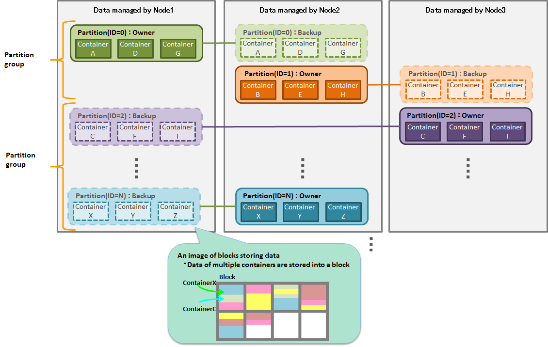
A partition is a data arrangement unit between clusters for managing the data movement to adjust the load balance between nodes and data multiplexing (replica) in case of a failure. Data replica is arranged in a node to compose a cluster on a partition basis.
A node that can be updated against a container inside a partition is known as an owner node and 1 node is allocated to each partition. A node that maintains replicas other than owner nodes is a backup node. Master data and multiple backup data exist in a partition, depending on the number of replicas set.
The relationship between a container and a partition is persistent and the partition which has a specific container is not changed. The relationship between a partition and a node is temporary and the autonomous data placement may cause partition migration to another node.
-
Partition group
A group of multiple partitions is known as a partition group.
Data maintained by a partition group is saved in an OS disk as a physical database file. A partition group is created with a number that depends on the degree of parallelism of the database processing threads executed by the node.
Data management unit
4 GridDB functions
Describes the data management functions, functions specific to the data model, operating functions and application development interfaces of GridDB.
4.1 Resource management
Besides the database residing in the memory, other resources constituting a GridDB cluster are perpetuated to a disk. The perpetuated resources are listed below.
-
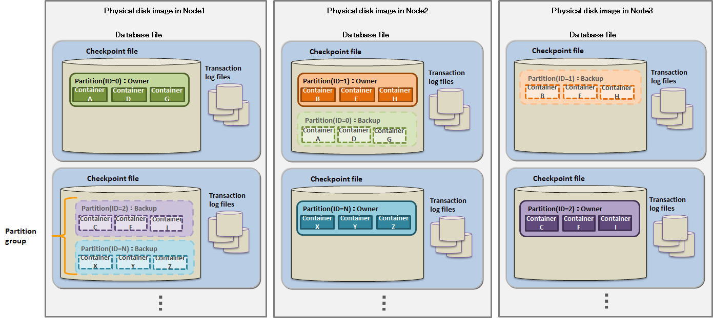
Database file
A database file is a file group consisting of transaction log file and checkpoint file that are perpetuated to a HDD or SSD. Transaction log file is updated everytime the GridDB database is updated or a transaction occurs, whereas the checkpoint file is written at a specified time interval.
-
Checkpoint file
A checkpoint file is the perpetuation of a partition group data from the memory to the disk at a specified time interval, as defined in the node definition file (/checkpoint/checkpointInterval). The size of checkpoint file increases along with the size of the data, however once the file gets expanded, its size will not decrease even if data such as containers or rows are deleted. In this case, GridDB reuses the free space instead.
-
Transaction log file
Transaction data that are written to the database in memory is perpetuated to the transaction log file by writing the data sequentially in a log format.
-
Definition file
There are 2 types of definition file, a parameter file (gs_cluster.json: hereinafter referred to as a cluster definition file) when composing a cluster, and a parameter file (gs_node.json: hereinafter referred to as a node definition file) to set the operations and resources of the node in the cluster. In addition, there is also a user definition file for GridDB administrator users.
-
Event log file
The operating log of the GridDB server is saved. Messages such as errors, warnings, etc. are saved.
-
Backup file
Backup data in the data file of GridDB is saved.
Database file
The layout of these resources can be defined in GridDB home (path specified in environmental variable GS_HOME). In the initial installation state, the /var/lib/gridstore directory is GridDB home, and the initial data of each resource is placed under this directory.
The initial configuration status is as follows.
/var/lib/gridstore/        # GridDB home directory
     admin/                # gs_admin home directory
     backup/               # Backup directory
     conf/                 # Definition files directory
          gs_cluster.json  # Cluster definition file
          gs_node.json     # Node definition file
          password         # User definition file
     data/                 # Database directory
     log/                  # Log directory
The location of GridDB home can be changed by setting the .bash_profile file of the OS user gsadm. If you change the location, please also move resources in the above directory accordingly.
The .bash_profile file contains two environment variables, GS_HOME and GS_LOG.
vi .bash_profile

# GridStore specific environment variables
GS_LOG=/var/lib/gridstore/log
export GS_LOG
GS_HOME=/var/lib/gridstore                   // GridDB home directory path
export GS_HOME
The database directory, backup directory and server event log directory can be changed by changing the settings of the node definition file as well.
In a system that has multiple disk drives, be sure to change the definition information in order to prevent loss of backup data during a disk failure.
See Parameters for the contents that can be set in the cluster definition file and node definition file.
4.2 User management
There are 2 types of GridDB user, an OS user which is created during installation and a GridDB user to perform operations/development in GridDB (hereinafter referred to a GridDB user).
4.2.1 OS user
An OS user has the right to execute operating functions in GridDB and a gsadm user is created during GridDB installation. This OS user is hereinafter referred to gsadm.
All GridDB resources will become the property of gsadm. In addition, all operating commands in GridDB are executed by a gsadm.
A check is conducted to see whether the user has the right to connect to the GridDB server and execute the operating commands. This authentication is performed by a GridDB user.
4.2.2 GridDB user
-
Administrator user and general user
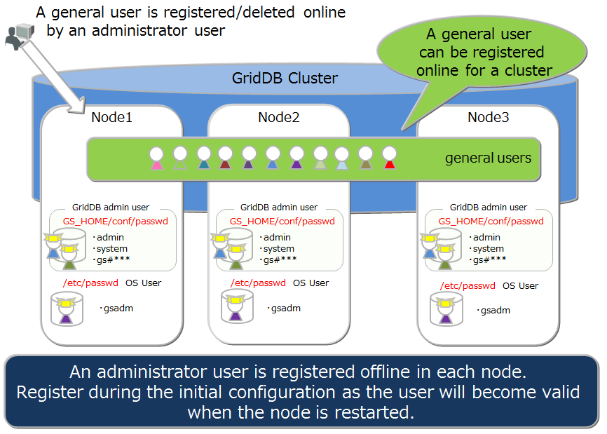
There are 2 types of GridDB user, an administrator user and a general user, which differ in terms of which functions can be used. Immediately after the installation of GridDB, 2 users, a system and an admin user, are registered as default administrator users.
An administrator user is a user created to perform GridDB operations while general users are users used by the application system.
For security reasons, administrator users and general users need to be used differently according to the usage purpose.
-
Creating a user
An administrator user can register or delete a gsadm, and the information is saved in the password file of the definition file directory as a GridDB resource. As an administrator user is saved/managed in a local file of the OS, it has to be placed so that the settings are the same in all the nodes constituting the cluster. In addition, administrator users need to be set up prior to starting the GridDB server. After the GridDB server is started, administrative users are not valid even if they are registered.
A general user can be created after an administrator user starts cluster operations in GridDB. A general user cannot be registered before the start of cluster services. A general user can only be registered using an operating command against a cluster as it is created after a cluster is composed in GridDB and maintained as management information in the GridDB database.
GridDB users
Since information is not communicated automatically among clusters, an administrator user needs to make the same settings in all the nodes and perform operational management such as determining the master management node of the definition file and distributing information from the master management node to all the nodes that constitute the cluster.
-
Rules when creating a user
There are naming rules to be adopted when creating a user name.
- Administrator user: Specify a user starting with “gs#”. After “gs#”, the name should be composed of only alphanumeric characters and the underscore mark. Since the name is not case-sensitive, gs#manager and gs#MANAGER cannot be registered at the same time.
- General user: Specify using alphanumeric characters and the underscore mark. However, the first character cannot be a number. In addition, since the name is not case-sensitive, user and USER cannot be registered at the same time. System and admin users cannot be created as default administrator users.
- Password: No restrictions on the characters that can be specified.
A string consisting of up to 64 characters can be specified for the user name and password.
4.2.3 Usable function
The operations that can be carried out by an administrator and a general user are shown below. Among the operations, commands which can be executed by a gsadm without using a GridDB user are marked with “✓✓”.
| Operations | Operating details | Operating tools used | gsadm | Administrator user | General user |
|---|---|---|---|---|---|
| Node operations | Starting a node | gs_startnode/gs_sh | ✓ | ✗ | |
| Stopping a node | gs_stopnode/gs_sh | ✓ | ✗ | ||
| Cluster operations | Building a cluster | gs_joincluster/gs_sh | ✓ | ✗ | |
| Adding a note to a cluster | gs_appendcluster/gs_sh | ✓ | ✗ | ||
| Detaching a node from a cluster | gs_leavecluster/gs_sh | ✓ | ✗ | ||
| Stopping a cluster | gs_stopcluster/gs_sh | ✓ | ✗ | ||
| User management | Registering an administrator user | gs_adduser | ✓✓ | ✗ | ✗ |
| Deleting an administrator user | gs_deluser | ✓✓ | ✗ | ✗ | |
| Changing the password of an administrator user | gs_passwd | ✓✓ | ✗ | ✗ | |
| Creating a general user | gs_sh | ✓ | ✗ | ||
| Deleting a general user | gs_sh | ✓ | ✗ | ||
| Changing the password of a general user | gs_sh | ✓ | ✓: Individual only | ||
| Database management | Creating/deleting a database | gs_sh | ✓ | ✗ | |
| Assigning/cancelling a user in the database | gs_sh | ✓ | ✗ | ||
| Data operations | Creating/deleting a container or table | gs_sh | ✓ | ✓: Only in the DB of the individual | |
| Registering data in a container or table | gs_sh | ✓ | ✓: Only in the DB of the individual | ||
| Searching for a container or table | gs_sh | ✓ | ✓: Only in the DB of the individual | ||
| Creating index to a container or table | gs_sh | ✓ | ✓: Only in the DB of the individual | ||
| Backup management | Creating a backup | gs_backup | ✓ | ✗ | |
| Restoring a backup | gs_restore | ✓✓ | ✗ | ✗ | |
| Displaying a backup list | gs_backuplist | ✓ | ✗ | ||
| System status management | Acquiring system information | gs_stat | ✓ | ✗ | |
| Changing system parameter | gs_paramconf | ✓ | ✗ | ||
| Data import/export | Importing data | gs_import | ✓ | ✓: Only in accessible object | |
| Exporting data | gs_export | ✓ | ✓: Only in accessible object |
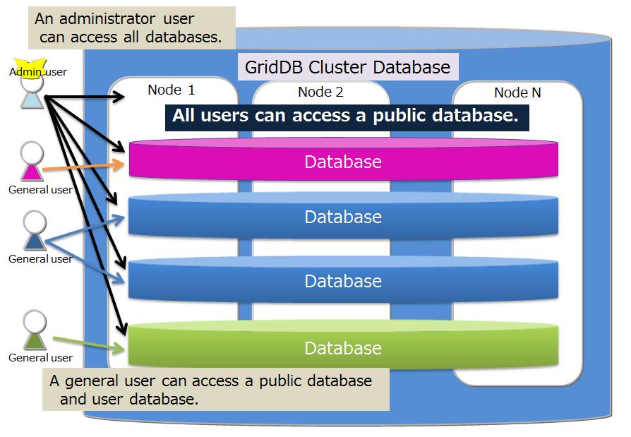
4.2.4 Database and user
Access to a cluster database in GridDB can be separated on a user basis. The separation unit is known as a database. The following is a cluster database in the initial state.
-
public
- The database can be accessed by all administrator user and general users.
- This database is used when connected without specifying the database at the connection point.
Multiple databases can be created in a cluster database. Creation of databases and assignment to users are carried out by an administrator user.
The rules for creating a database are as shown below.
- The maximum no. of users and the maximum no. of databases that can be created in a cluster database is 128.
- A string consisting of alphanumeric characters, the underscore mark, the hyphen mark, the dot mark, the slash mark and the equal mark can be specified for the database. However, the first character cannot be a number.
- A string consisting of 64 characters can be specified for the database name.
- Although the case sensitivity of the database name is maintained, a database which has the same name when it is not case-sensitive cannot be created.
- “public” and “information_schema” cannot be specified for default DB.
Only assigned general users and administrator users can access the database. Administrator user can access all databases. The following rules apply when assign a general user to a database.
- Only 1 general user can be assigned to 1 database
- Multiple databases can be assigned to 1 user
Database and users
4.3 Data management function
To register and search for data in GridDB, a container (table) needs to be created to store the data. It is called a container when operating with NoSQL I/F, and a table when operating with NewSQL I/F. This section describes the data types that can be registered in a container (table), data size, index and data management functions.
The naming rules for containers (tables) are the same as those for databases.
- A string consisting of alphanumeric characters, the underscore mark, the hyphen mark, the dot mark, the slash mark and the equal mark can be specified. However, the first character cannot be a number.
- Although the case sensitivity of the name is maintained, a container (table) which has the same name when it is not case-sensitive cannot be created.
4.3.1 Container (table) data type
There are 2 container (table) data types.
A timeseries container (timeseries table) is a data type which is suitable for managing hourly data together with the occurrence time while a collection (table) is suitable for managing a variety of data.
The schema can be set in a container (table).
The basic data types that can be registered in a container (table) are the basic data type and array data type .
4.3.1.1 Basic data types
Describes the basic data types that can be registered in a container (table). A basic data type cannot be expressed by a combination of other data types.
| Data type | Description |
|---|---|
| BOOL | True or false |
| STRING | Composed of an arbitrary number of characters using the unicode code point |
| BYTE | Integer value from -2^{7} to 2^{7}-1 (8 bits) |
| SHORT | Integer value from -2^{15} to 2^{15}-1 (16 bits) |
| INTEGER | Integer value from -2^{31} to 2^{31}-1 (32 bits) |
| LONG | Integer value from -2^{63} to ら2^{63}-1 (64 bits) |
| FLOAT | Single-precision data type (32 bits) Floating-point number defined in IEEE754 |
| DOUBLE | Double-precision data type (64 bits) Floating-point number defined in IEEE754 |
| TIMESTAMP | Data type expressing the date and time Data format maintained in the database is UTC, and accuracy is in milliseconds |
| GEOMETRY | Data type to represent a space structure |
| BLOB | Data type for binary data such as images, audio, etc. |
The following restrictions apply to the size of the data that can be managed for STRING, GEOMETRY and BLOB data. The restriction value varies according to the block size which is the input/output unit of the database in the GridDB definition file (gs_node.json).
| Data type | Block size (64KB) | Block size (1MB) |
|---|---|---|
| STRING | Maximum 31KB (equivalent to UTF-8 encode) | Maximum 128KB (equivalent to UTF-8 encode) |
| GEOMETRY | Maximum 31KB (equivalent to the internal storage format) | Maximum 128KB (equivalent to the internal storage format) |
| BLOB | Maximum 1GB - 1Byte | Maximum 1GB - 1Byte |
[Memo]
- GEOMETRY is not supported in a table (operation by NewSQL I/F). Please use GEOMETRY in a container (operation by NoSQL I/F).
4.3.1.2 HYBRID
A data type composed of a combination of basic data types that can be registered in a container. The only hybrid data type in the current version is an array.
-
ARRAY
Expresses an array of values. Among the basic data types, only GEOMETRY and BLOB data cannot be maintained as an array. The restriction on the data volume that can be maintained in an array varies according to the block size of the database.
Data type Block size (64KB) Block size (1MB) Number of arrays 4000 65000 [Memo]
The following restrictions apply to TQL operations in an array column.
-
Although the i-th value in the array column can be compared, calculations (aggregation) cannot be performed on all the elements.
-
*(Example) When column A is an array and assumed to be defined
- The elements in an array such as select * where ELEMENT (0, column A) > 0 can be specified and compared. However, the variable in the ELEMNT "0" section cannot be specified.
- Aggregation such as select SUM (column A) cannot be carried out.
-
*(Example) When column A is an array and assumed to be defined
-
Although the i-th value in the array column can be compared, calculations (aggregation) cannot be performed on all the elements.
4.3.2 GEOMETRY-type (Spatial-type)
GEOMETRY data are widely used in map information systems, etc. This type can only be specified for container and not be supported for table.
For GEOMETRY, data is written in WKT (Well-known text). WKT is formulated by the Open Geospatial Consortium (OGC), a nonprofit organization promoting standardization of information on geospatial information.
The following WKT format data can be stored in the GEOMETRY column.
-
POINT
- Point represented by two or three-dimensional coordinate.
- Example) POINT(0 10 10)
-
LINESTRING
- Set of straight lines in two or three-dimensional space represented by two or more points.
- Example) LINESTRING(0 10 10, 10 10 10, 10 10 0)
-
POLYGON
- Closed area in two or three-dimensional space represented by a set of straight lines.
- Example) POLYGON((0 0,10 0,10 10,0 10,0 0)), POLYGON((35 10, 45 45, 15 40, 10 20, 35 10),(20 30, 35 35, 30 20, 20 30))
-
POLYHEDRALSURFACE
- Area in the three-dimensional space represented by a set of the specified area.
- Example) POLYHEDRALSURFACE(((0 0 0, 0 1 0, 1 1 0, 1 0 0, 0 0 0)), ((0 0 0, 0 1 0, 0 1 1, 0 0 1, 0 0 0)), ((0 0 0, 1 0 0, 1 0 1, 0 0 1, 0 0 0)), ((1 1 1, 1 0 1, 0 0 1, 0 1 1, 1 1 1)), ((1 1 1, 1 0 1, 1 0 0, 1 1 0, 1 1 1)), ((1 1 1, 1 1 0, 0 1 0, 0 1 1, 1 1 1)))
-
QUADRATICSURFACE
- Two-dimensional curved surface in a three-dimensional space represented by defining equation f(X) = <AX, X> + BX + c.
Operations using GEOMETRY can be executed with API or TQL.
With TQL, management of two or three-dimensional spatial structure is possible. Generating and judgement function are also provided.
SELECT * WHERE ST_MBRIntersects(geom, ST_GeomFromText('POLYGON((0 0,10 0,10 10,0 10,0 0))'))
See “GridDB API Reference” (GridDB_API_Reference.html) for details of the functions of TQL.
4.3.3 Container (table) ROWKEY
A ROWKEY is the data set in the row of a container. The uniqueness of a row with a set ROWKEY is guaranteed.
In NewSQL I/F, ROWKEY is called as PRIMARY KEY.
A ROWKEY can be set in the first column of the row. (This is set in Column No. 0 since columns start from 0 in GridDB.)
-
For a timeseries container (timeseries table)
- ROWKEY (PRIMARY KEY) is a TIMESTAMP
- Must be specified.
-
For a collection (table)
- A ROWKEY (PRIMARY KEY) is either a STRING, INTEGER, LONG or TIMESTAMP column.
- Need not be specified.
A default index prescribed in advance according to the column data type can be set in a column set in ROWKEY (PRIMARY KEY).
In the current version, the default index of all STRING, INTEGER, LONG or TIMESTAMP data that can be specified in a ROWKEY (PRIMARY KEY) is the TREE index.
4.3.4 Container (table) index
A condition-based search can be processed quickly by creating an index for the columns of a container (table).
There are 3 types of index - hash index (HASH), tree index (TREE) and space index (SPATIAL). A hash index is used in an equivalent-value search when searching with a query in a container. Besides equivalent-value search, a tree index is used in comparisons including the range (bigger/same, smaller/same etc.).
The index that can be set differs depending on the container (table) type and column data type.
-
HASH INDEX
- An equivalent value search can be conducted quickly but this is not suitable for searches that read the rows sequentially.
-
Columns of the following data type can be set in a collection. Cannot be set in a timeseries container, a table, and a timeseries table.
- STRING
- BOOL
- BYTE
- SHORT
- INTEGER
- LONG
- FLOAT
- DOUBLE
- TIMESTAMP
-
TREE INDEX
- Besides equivalent-value search, a tree index is used in comparisons including the range (bigger/same, smaller/same etc.).
-
This can be used for columns of the following data type in any type of container (table), except for columns corresponding to a rowkey in a timeseries container (timeseries table).
- STRING
- BOOL
- BYTE
- SHORT
- INTEGER
- LONG
- FLOAT
- DOUBLE
- TIMESTAMP
-
SPATIAL INDEX
- Can be used for only GEOMETRY columns in a collection. This is specified when conducting a spatial search at a high speed.
Although there are no restrictions on the no. of indices that can be created in a container, creation of an index needs to be carefully designed. An index is updated when the rows of a configured container are inserted, updated or deleted. Therefore, when multiple indices are created in a column of a row that is updated frequently, this will affect the performance in insertion, update or deletion operations.
An index is created in a column as shown below.
- A column that is frequently searched and sorted
- A column that is frequently used in the condition of the WHERE section of TQL
- High cardinality column (containing few duplicated values)
4.3.5 Timeseries container (timeseries table)
In order to manage data from a sensor etc. occurring at a high frequency, data is placed in accordance with the data placement algorithm (TDPA: Time Series Data Placement Algorithm) making maximum effective use of the memory . In a timeseries container (timeseries table), memory is allocated while classifying internal data by its periodicity. When hint information is given in an affinity function, the placement efficiency rises further. Expired data in a timeseries container is released at almost zero cost while being expelled to a disk where necessary.
A timeseries container (timeseries table) has a TIMESTAMP ROWKEY (PRIMARY KEY).
4.3.5.1 Expiry release function
In a timeseries data, an expiry release function and the data retention period can be set so that when the period set is exceeded, the data will be released (deleted).
The settings refer to the deadline unit and deadline, and no. of divisions when the data is released during timeseries container (timeseries table) creation. The settings of a timeseries container (timeseries table) that has been created cannot be changed.
The deadline can be set in day/hour/minute/sec/millisec units. The year unit and month unit cannot be specified. The current time used in determining whether the valid period has expired is dependent on the execution environment of each node in GridDB. Therefore, if the GridDB node time is faster than the client time due to a network delay or a deviation in the time setting of the execution environment, or if a row prior to expiry is no longer accessible, or conversely if only the client time is faster, the expired row may be accessible. We recommend that a value larger than the minimum required time is set in order to avoid unintended loss of rows.
An expired row is deemed as non-existent and is no longer subject to row operations such as search and update.
Expired rows are physically deleted based on the number of divisions for the valid period (number of divisions when the data is deleted).
For example, if the valid period is 720 days and the specified number of divisions is 36, although data access will be immediately disabled upon passing the 720-day mark, the data will only be deleted after 20 days have passed from the 720 days. 20 days’ worth of physical data is deleted together.
The number of divisions is specified when creating a timeseries container (timeseries table).
4.3.5.2 Compression function
In timeseries container (timeseries table), data can be compressed and held. Data compression can improve memory usage efficiency. Compression options can be specified when creating a timeseries container (timeseries table).
However, the following row operations cannot be performed on a timeseries container (timeseries table) for which compression options are specified.
- Updating a specified row.
- Deleting a specified row.
- Inserting a new row when there is a row at a later time than the specified time.
The following compression types are supported:
- HI: thinning out method with error value
- SS: thinning out method without error value
- NO: no compression.
The explanation of each option is as follows.
- Thinning out method with error value (HI)
HI compression is illustrated below. When the previous and the following registered data lies in the same slope, the current data, which is represented by a row is omitted. The condition of the slope can be specified by the user.
The row data is omitted only when the specified column satisfies the condition and the values of the other columns are the same as the previous data. The condition is specified by the error width (Width).
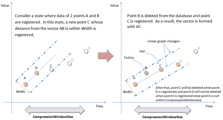
Compression of timeseries container (timeseries table)
Compression can be enabled to the following data types:
- LONG
- INTEGER
- SHORT
- BYTE
- FLOAT
- DOUBLE
Since lossy compression is used, data omitted by the compression cannot be restored to its original value.
Omitted data will be restored without error value at the process of interpolate and sample processing.
- Thinning out method without error value (SS)
With SS type, the row with the same data as the row registered just before and immediately after will be omitted. Omitted data will be restored without error value at the process of interpolate and sample processing.
4.3.5.3 Calculation of a timeseries container
There are calculations to perform time correction in addition to calculations to aggregate containers in a timeseries container (timeseries table).
-
Aggregate operations
When performing an aggregate operation on a container, the start and end time needs to be specified before applying the aggregate operation on a row set or specific column.
The functions of the aggregate operation are as follows:
-
AVG(column)
Returns the average value of the specified column.
-
COUNT(*)
Return the number of rows satisfying a given condition(s).
-
MAX(column)
Returns the largest value in the specified column.
-
MIN(column)
Returns the smallest value in the specified column.
-
STDDEV(column)
Returns the standard deviation of values in the specified column.
-
SUM((column)
Return the sum of values in the specified column.
-
VARIANCE(column)
Returns the variance of values in the specified column.
-
AVG(column)
-
Aggregate operation specific to a timeseries container (timeseries table)
In a timeseries container (timeseries table), the calculation is performed with the data weighted at the time interval of the sampled data. In other words, if the time interval is long, the calculation is carried out assuming the value is continued for an extended time.
The functions of the aggregate operation specific to a timeseries container (timeseries table) is as follows:
-
TIME_AVG
Returns the average weighted by a time-type key of values in the specified column.
The weighted average is calculated by dividing the sum of products of sample values and their respective weighted values by the sum of weighted values. Only a numeric-type Column can be specified. The method for calculating a weighted value is as shown above.
The details of the calculation method are shown in the figure:
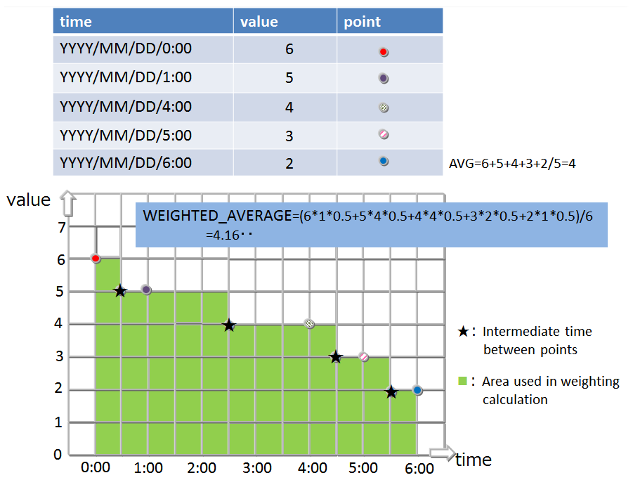
Aggregation of weighted values (TIME_AVG)
-
TIME_AVG
4.3.6 Selection and interpolation of a timeseries container (timeseries table)
Time data may deviate slightly from the expected time due to the timing of the collection and the contents of the data to be collected. Therefore when conducting a search using time data as a key, a function that allows data around the specified time to be acquired is also required.
The functions for searching the timeseries container (timeseries table) and acquiring the specified row are as follows:
-
TIME_NEXT(*, timestamp)
Selects a time-series row whose timestamp is identical with or just after the specified timestamp.
-
TIME_NEXT_ONLY(*, timestamp)
Select a time-series row whose timestamp is just after the specified timestamp.
-
TIME_PREV(*, timestamp)
Selects a time-series row whose timestamp is identical with or just before the specified timestamp.
-
TIME_PREV_ONLY(*, timestamp)
Selects a time-series row whose timestamp is just before the specified timestamp.
In addition, the functions for interpolating the values of the columns are as follows:
-
TIME_INTERPOLATED(column, timestamp)
Returns a specified column value of the time-series row whose timestamp is identical with the specified timestamp, or a value obtained by linearly interpolating specified column values of adjacent rows whose timestamps are just before and after the specified timestamp, respectively.
-
TIME_SAMPLING(*|column, timestamp_start, timestamp_end, interval, DAY|HOUR|MINUTE|SECOND|MILLISECOND)
Takes a sampling of Rows in a specific range from a given start time to a given end time.
Each sampling time point is defined by adding a sampling interval multiplied by a non-negative integer to the start time, excluding the time points later than the end time.
If there is a Row whose timestamp is identical with each sampling time point, the values of the Row are used. Otherwise, interpolated values are used.
4.3.7 Affinity function
An affinity is a function to connect related data. There are 2 types of affinity function in GridDB, data affinity and node affinity.
4.3.7.1 Data affinity function
A data affinity is a function to raise the memory hit rate by arranging highly correlated data in the same block and localizing data access. By raising the memory hit ratio, the no. of memory mishits during data access can be reduced and the throughput can be improved. By using data affinity, even machines with a small memory can be operated effectively.
The data affinity settings provide hint information as container properties when creating a container (table). The characters that can be specified for the hint information are restricted by naming rules that are similar to those for the container (table) name. Data with the same hint information is placed in the same block as much as possible.
Data affinity hints are set separately by the data update frequency and reference frequency. For example, consider the data structure when system data is registered, referenced or updated by the following operating method in a system that samples and refers to the data on a daily, monthly or annual basis in a monitoring system.
- Data in minutes is sent from the monitoring device and saved in the container created on a monitoring device basis.
- Since data reports are created daily, one day’s worth of data is aggregated from the data in minutes and saved in the daily container
- Since data reports are created monthly, daily container (table) data is aggregated and saved in the monthly container
- Since data reports are created annually, monthly container (table) data is aggregated and saved in the annual container
- The current space used (in minutes and days) is constantly updated and displayed in the display panel.
In GridDB, instead of occupying a block in a container unit, data close to the time is placed in the block. Therefore, refer to the daily container (table) in 2., perform monthly aggregation and use the aggregation time as a ROWKEY (PRIMARY KEY). The data in 3. and the data in minutes in 1. may be saved in the same block.
If the memory is small and the data is so big that all the monitoring data cannot be stored in the memory, when the aggregation process in 4. is carried out on an annual basis, the block is divided and data placed in 3. is placed in the memory. As a result, data that you want to monitor may get swapped out as the data read may not be the latest e.g. data in 1. which is not required all the time is driven out of the memory.
In this case, by providing hints to the container (table) according to the container (table) access frequency using a data affinity e.g. on a minute, daily or monthly basis, etc., data with a low access frequency and data with a high access frequency is separated into different blocks when the data is placed.
In this way, data can be placed to suit the usage scene of the application by the data affinity function.
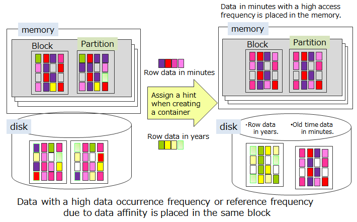
Data Affinity
4.3.7.2 Node affinity function
Node affinity is a function to reduce the network load when accessing data by arranging highly correlated containers and tables in the same node. Although there is no container JOIN operation In the TQL of a NoSQL product, a table JOIN operation can be described in the SQL of a SQL product. When joining a table, the network access load of a table placed in another node of the cluster can be reduced. In addition, since concurrent processing using multiple nodes is no longer possible, there is no effect on shortening the turnaround time. Nonetheless, throughput may still rise due to a reduction in the network load.
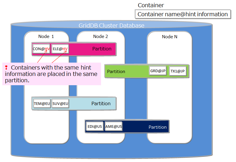
Placement of container/table based on node affinity
To use the node affinity function, hint information is given in the container (table) name when the container (table) is created. A container (table) with the same hint information is placed in the same partition. Specify the container name as shown below.
- Container (table) name@node affinity hint information
The naming rules for node affinity hint information are the same as the naming rules for the container (table) name.
4.3.8 Table partitioning (GridDB AE/VE)
In order to improve the operation speed of applications connected to multiple nodes of the GridDB cluster, it is important to arrange the data to be processed in memory as much as possible. For huge table with a large number of rows, by distributing rows of the table to multiple nodes, processors and memory of multiple nodes can be effectively used. Distributed rows are stored in the internal containers called "data partition". The allocation of each row to the data partition is determined by a "partitioning key" column specified at the time of the table creation.
GridDB supports hash partitioning, interval partitioning and interval-hash partitioning as table partitioning methods.
Table partitioning is a function only for GridDB AE/VE. Creating and Deleting tables can be performed only through the NewSQL interface. Data registration, update and search can be performed through the NewSQL/NoSQL interface. (There are some restrictions. See TQL and SQL for the details.)
-
Data registration
When data is registered into a table, the data is stored in the appropriate data partition according to the partitioning key value and the partitioning method. It is not possible to specify a data partition to be stored.
-
Index
When creating an index on a table, a local index for each data partition is created. It is not possible to create a global index for the whole table.
-
Data handling
An error occurs for updating the partitioning key value. If updating the partitioning key is needed, delete and reregister the data.
-
Functions of timeseries tables
The expiry release function can be used for partitioned timeseries tables. The compression function cannot be used for the tables.
-
Notes
When specifying the column as a partitioning key other than the primary key, the primary key constraint is ensured in each data partition, but it is not ensured in the whole table. So, the same value may be registered in multiple rows of a table.
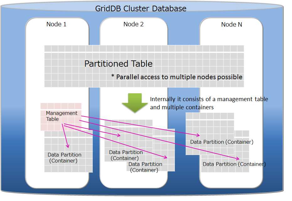
Table partitioning
4.3.8.1 Benefits of table partitioning
Dividing a large amount of data through a table partitioning is effective for efficient use of memory and for performance improvement in data search which can select the target data.
-
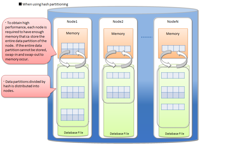
efficient use of memory
In data registration and search, data partitions required for the processing are loaded into memory. Other data partitions, not target to the processing, are not loaded. So when the data to be processed is locally concentrated on some data partitions, the amount of loading data is reduced. The frequency of swap-in and swap-out is decreased and the performance is upgraded.
-
selecting target data in data search
In data search, only data partitions matching the search condition are selected as the target data. Unnecessary data partitions are not accessed. This function is called "pruning". Because the amount of accessed data reduces, the search performance is upgraded. Search conditions which can enable the pruning are different depending on the type of the partitioning.
The followings describe the behaviors on the above items for both cases in not using the table partitioning and in using the table partition.
When a large amount of data is stored in single table which is not partitioned, all the required data might not be able to be placed on main memory and the performance might be degraded by frequent swap-in and swap-out between database files and memory. Particularly the degradation is significant when the amount of data is much larger than the memory size of a GridDB node. And data accesses to that table concentrate on single node and the parallelism of database processing decreases.
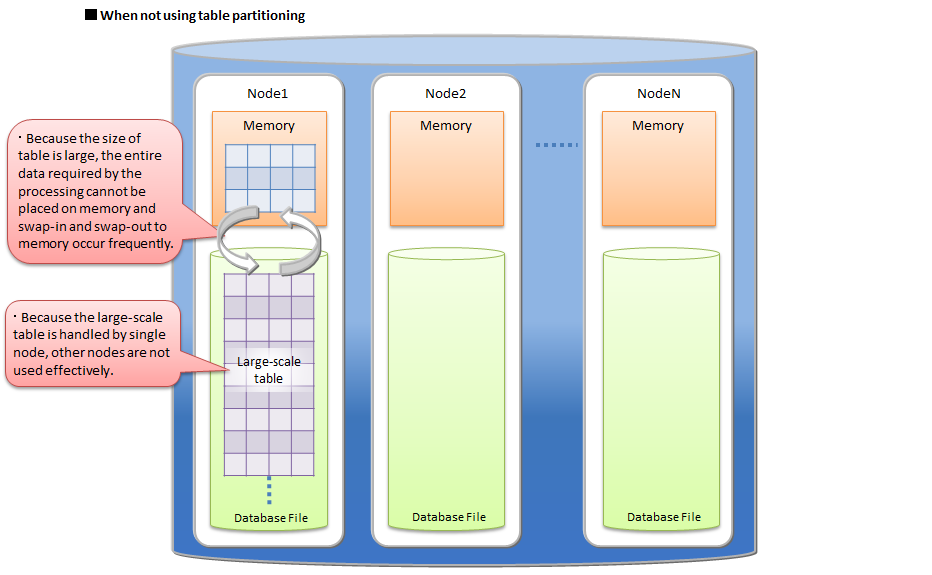
When not using table partitioning
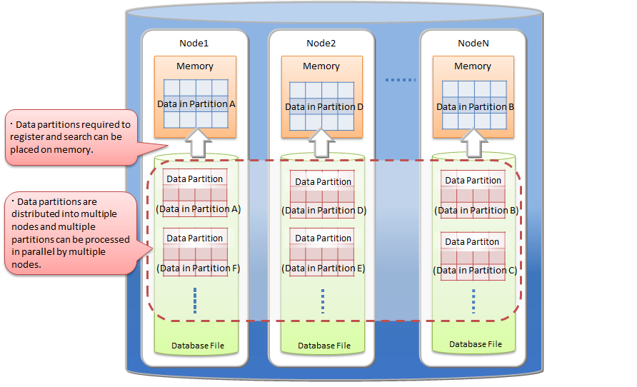
By using a table partitioning, the large amount of data is divided into data partitions and those partitions are distributed on multiple nodes.
In data registration and search, only necessary data partitions for the processing can be loaded into memory. Data partitions not target to the processing are not loaded. Therefore, in many cases, data size required by the processing is smaller than for a not partitioned large table and the frequency of swap-in and swap-out decreases. By dividing data into data partitions equally, CPU and memory resource on each node can be used more effectively.
In addition data partitions are distributed on nodes, so parallel data access becomes possible.
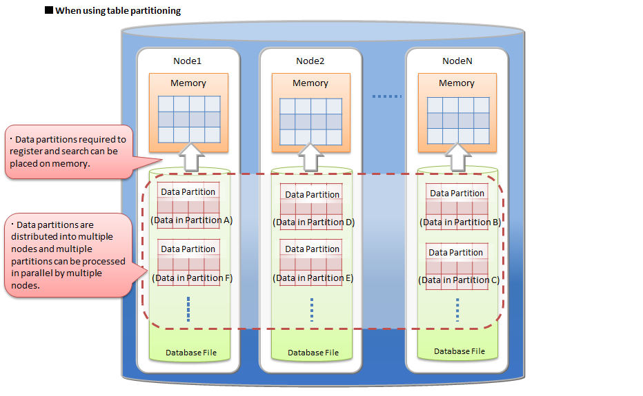
When using table partitioning
4.3.8.2 Hash partitioning
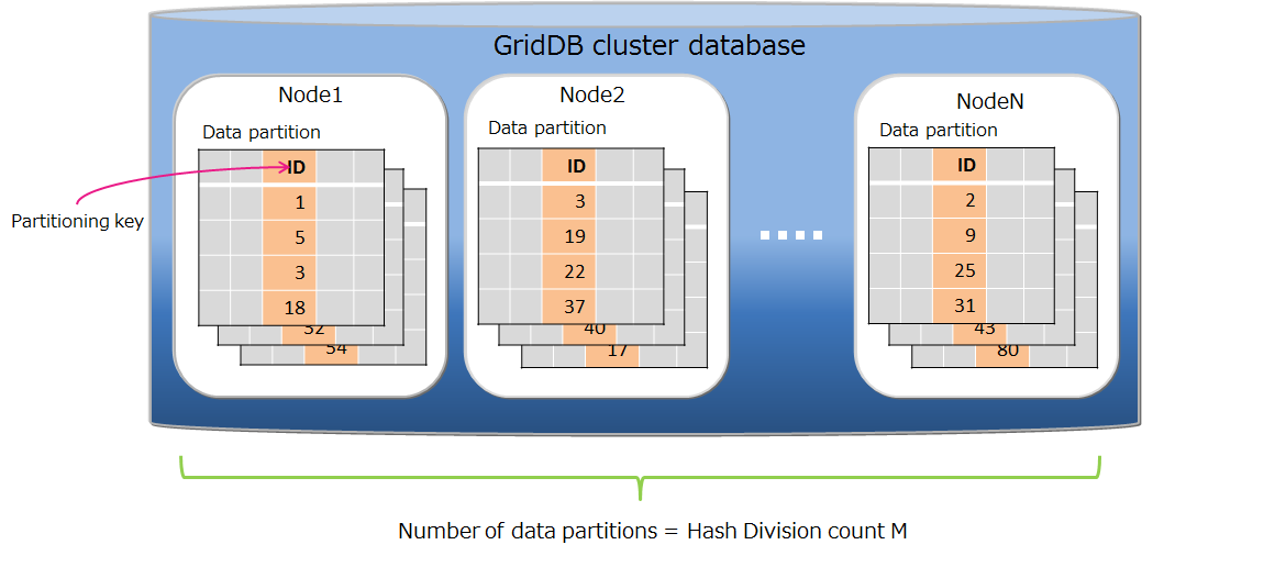
The rows are evenly distributed in the data partitions based on the hash value.
Also, when using an application system that performs data registration at a high frequency, the access will concentrate at the end of the table and may lead to a bottleneck. Since multiple table can be prepared by hash partitioning, it can be used to distribute the access.
A hash function that returns an integer from 1 to N is defined by specifying the partition key column and division number N, and division is performed based on the returned value.
Hash partitioning
-
Data partitioning
By spceifying the partitioning key and the division count M, a hash function that returns 1〜M is defined, and data partitioning is performed by the hash value. The maximum hash value is 1024.
-
Partitioning key
There is no limitation for the column type of a partitioning key.
-
Creation of data partitions
Specified number of data partitions are created automatically at the time of the table creation. It is not possible to change the number of data partitions. The table re-creation is needed for changing the number.
-
Deletion of a table
It is not possible to delete only a data partition.
By deleting a hash partitioned table, all data partitions that belong to it are also deleted
-
Pruning
In key match search on hash partitioning, by pruning, the search accesses only data partitions which match the condition. So the hash partitioning is effective for performance improvement and memory usage reduction in that case.
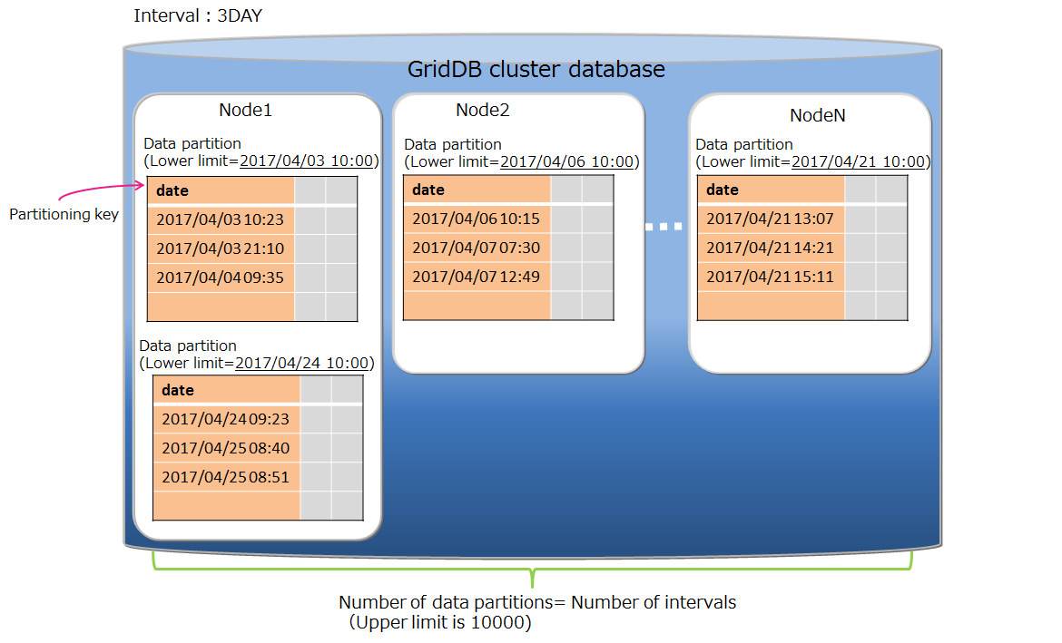
4.3.8.3 Interval partitioning
In the interval partitioning, the rows in a table are divided by the specified interval value and is stored in data partitions. The range of each data partition (from the lower limit value to the upper limit value) is automatically determined by the interval value.
The data in the same range are stored in the same data partition, so for the continuous data or for the range search, the operations can be performed on fewer memory.
Interval partitioning
-
Data partitioning
Data partitioning is performed by the interval value. The possible interval values are differnt depending on the partitioning key type.
- BYTE: 1~127
- SHORT: 1~32767
- INTEGER: 1~2147483647
- LONG: 1000~9223372036854775807
- TIMESTAMP: 1~
When the partitioning key type is TIMESTAMP, it is necessary to specify the interval unit as 'DAY'.
-
Partitioning key
Data types that can be specified as a partitioning key are BYTE, SHORT, INTEGER, LONG and TIMESTAMP. The partitioning key is a column that needs to have "NOT NULL" constraint.
-
Creation of data partitions.
Data partitions are not created at the time of creating the table. When there is no data partition for the registered row, a new data partition is automatically created.
The upper limit of the number of the data partitions is 10000. When the number of the data partitions reaches the limit, the data registration that needs to create a new data partition causes an error. For that case, delete unnecessary data partitions and reregister the data.
It is desired to specify the interval value by considering the range of the whole data and the upper limit, 10000, for the number of data partitions. If the interval value is too small to the range of the whole data and too many data partitions are created, the maintenance of deleting unnecessary data partitions is required frequently.
-
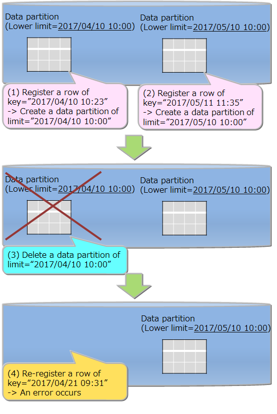
Deletion of data partitions
Each data partition can be deleted. The data partition that has been deleted cannot be recreated. All registration operations to the deleted data partition cause an error. Before deleting the data partition, check its data range by a metatable. See the SQL reference manual for the details of metatable operations.
By deleting an interval partitioned table, all data partitions that belong to it are also deleted.
If the expiry release function is set, the data partition that becomes empty for the expiration is not deleted automatically. All data partitions are processed for the data search on the whole table, so the search can be performed efficiently by deleting unnecessary data partitions beforehand.
-
Maintenance of data partitions
In the case of reaching the upper limit, 10000, for the number of data partitions or existing unnecessary data partitions, the maintenance by deleting data partitions is needed.
-
How to check the number of data partitions
It can be check by search the metatable that holds the data about data partitions. See "GridDB Advanced Edition SQL reference" (GridDB_AE_SQL_Reference.pdf) for the details.
-
How to delete data partitions
They can be deleted by specifying the lower limit value in the data partition. See "GridDB Advanced Edition SQL reference" (GridDB_AE_SQL_Reference.pdf) for the details.
-
How to check the number of data partitions
Examples of interval partitioned table creation and deletion
-
Pruning
By specifying a partitioning key as a search condition in the WHERE clause, the data partitions corresponding the specified key are only referred for the search, so that the processing speed and the memory usage are improved.
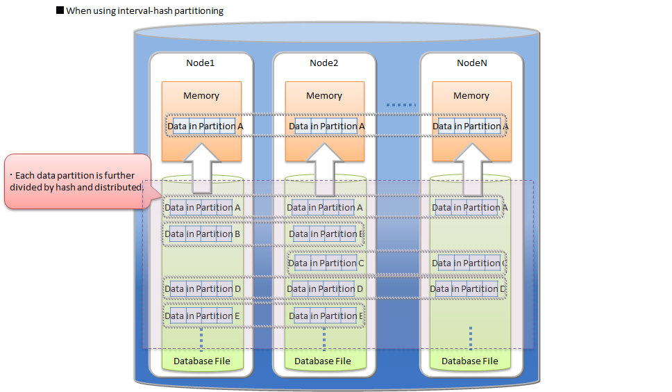
4.3.8.4 Interval-hash partitioning
The interval-hash partitioning is a combination of the interval partitioning and the hash partitioning. First the rows are divided by the interval partitioning, and further each division is divided by hash partitioning. The number of data partitions is obtained by multiplying the interval division count and the hash division count together.
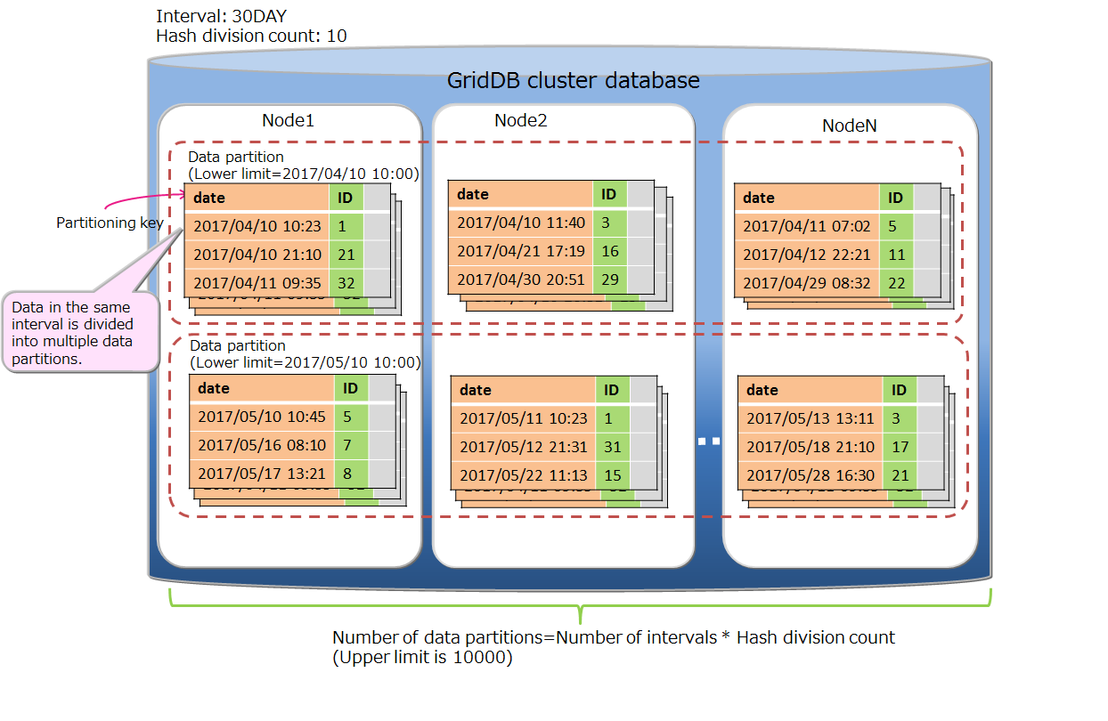
Interval-hash partitioning
The rows are distributed to multiple nodes appropriately through the hash partitioning on the result of the interval partitioning. On the other hand, the number of data partitions increases, so that the overhead of searching on the whole table also increases. Please judge to use the partitioning by considering its data distribution and search overhead.
The basic functions of the interval-hash partitionig are the same as the functions of interval partitioning and the hash partitioning. The items specific for the interval-hash partitionig are as follows.
-
Data partitioning
The possible interval values of LONG are different from the interval partitioning.
- BYTE: 1~127
- SHORT: 1~32767
- INTEGER: 1~2147483647
- LONG: 1000*the hash division count~9223372036854775807
- TIMESTAMP: 1~
-
Number of data partitions
Including partitions divided by hash, the upper limit of number of data partitions is 10000. The behavior and requiring maintenance when the limit has been reached are same as interval partitioning.
-
Deletion of data partitions
A group of data partitions which have the same range can be deleted. It is not possible to delete only a data partition divided by the hash partitioning.
4.3.8.5 Selection criteria of table partitioning type
Hash, interval and interval-hash are supported as a type of table partitioning by GridDB.
A column which is used in conditions of search or data access must be specified as a partitioning key for dividing the table. If a width of range that divides data equally can be determined for values of the partitioning key, interval or interval-hash is suitable. Otherwise hash should be selected.
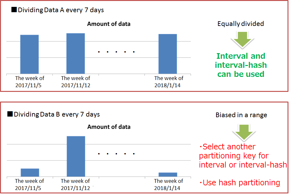
Data range
-
Interval partitioning, interval-hash partitioning
If an interval, a width of range to divide data equally, can be determined beforehand, interval partitioning is suitable. In the query processing on interval partitioning, by partitioning pruning, the result is acquired from only the data partitions matching the search condition, so the performance is improved.
Interval partitioning
Therefore, when using interval partitioning, by selecting an appropriate interval value based on frequently registered or searched data range in application programs, required memory size is reduced. For example, when most recent range in time series data, such as sensing data, is accessed frequently, by specifying the width of the access range as the interval of table partitioning, data processing is performed only on the memory which has the target data partition and the search performance is not degraded.
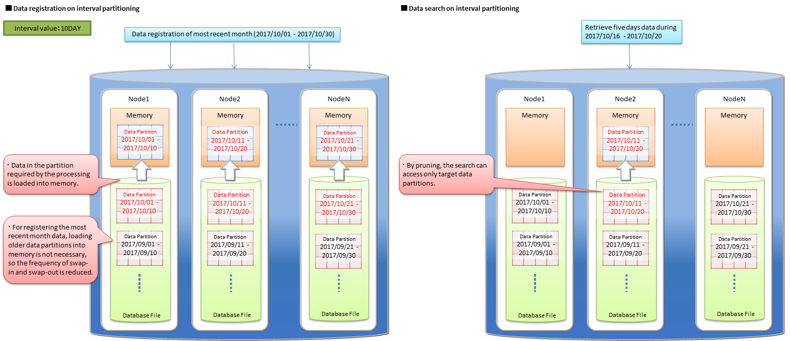
Examples of data registration and search on interval partitioning
Further by using interval-hash partitioning, data in each interval is distributed to multiple nodes equally, so accesses to the same data partition can also be performed in parallel.
Interval-hash partitioning
-
Hash partitioning
When the characteristics of data to be stored is not clear or finding the interval value, which can divide the data equally, is difficult, hash partitioning should be selected. By specifying a column holding unique values as a partitioning key, uniform partitioning for a large amount of data is performed easily.
Hash partitioning
When using hash partitioning, the parallel access to the entire table and the partitioning pruning which is enabled only for exact match search can be performed, so the system performance can be improved. But, to obtain high performance, each node is required to have enough memory that can store the entire data partition of the node.
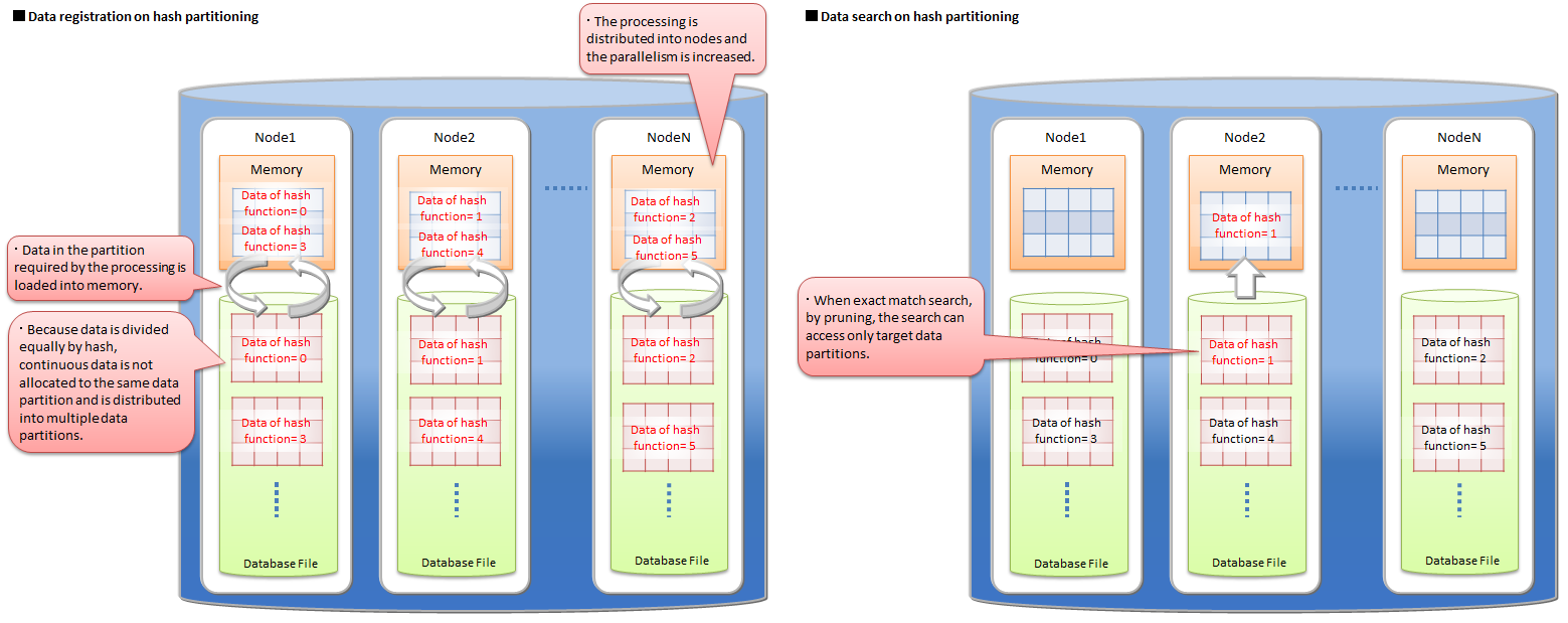
Examples of data registration and search on hash partitioning
4.3.9 Container placement information
Containers (tables) and partitioned tables in a GridDB cluster are automatically distributed to each node. By using operation management tools or SQL, it is possible to check which container (table) is placed on each node.
This function is used to:
- check containers placed on a node when the database size of each node is not balanced.
- find backup location of the node where specified container is placed on.
[Memo]
- See the "Data model" for the description of the container and partition.
- When the autonomous data placement is executed by a node down or a node failure, the placement of containers may be changed. The placement of containers is not persistent.
The placement information of containers (tables) is checked by the following methods.
4.3.9.1 Getting container (table) list of node
To get container (table) list of a node, use "Container list screen" of integrated operation control GUI (gs_admin).
- Login to gs_admin.
- After selecting the "ClusterTree" tab on the left tree view and selecting a node, click "Container" tab on the right frame.
- Container list placed on the node is displayed.
[Memo]
- For partitioned table, the management table is only displayed. Data partitions are not displayed.
4.3.9.2 Checking owner node of container (table)
To check node where specified container is placed on, use gs_sh and operation command (gs_parition).
- Perform gs_sh subcommand "showcontainer" to check ID of the partition which has specified container. The partition ID is displayed as "Partition ID".
- Perform gs_sh subcommand "configcluster" to check master node. "M" is displayed as "Role" for the master node.
- Perform the command "gs_partition" to the master node with an argument specifying the partition ID. The "/owner/address" in the displayed JSON shows the owner node of the container (table).
[Example]
-
Getting a particular partition information.
$ gs_partition -u admin/admin -n 5
[
    {
        "backup": [],
        "catchup": [],
        "maxLsn": 300008,
        "owner": {
            "address": "192.168.11.10",    -> The IP address of the owner node is 192.168.11.10.
            "lsn": 300008,
            "port": 10010
        },
        "pId": "5",
        "status": "ON"
    }
]
[Points to note]
- When performing the gs_partition on a node except the master node, the information of the partition may not be correct.
[Memo]
- When specifying partitioned table, the placement information of the management table is only displayed. The placement information of the data partitions is not displayed.
4.3.9.3 Checking node of data partition (AE only)
To get the internal container (data partition) locations of each partitioned table, use the metatable. The metatable can be referenced by SQL.
Perform SQL on the metatable "#table_partitions" using the "SQL screen" of the integrated operation control management GUI (gs_admin) or the "sql" subcommand of the interpreter (gs_sh).
The list of data partitions and their node addresses is displayed.
[Example]
-
Displaying the addresses of the nodes where each data partition of partitioned table "hashTable" is placed on.
select DATABASE_NAME, TABLE_NAME, CLUSTER_NODE_ADDRESS from "#table_partitions" where TABLE_NAME='hashTable';

DATABASE_NAME,TABLE_NAME,CLUSTER_NODE_ADDRESS
public,hashTable,192.168.11.10:20001
public,hashTable,192.168.11.12:20001
public,hashTable,192.168.11.11:20001
public,hashTable,192.168.11.13:20001
public,hashTable,192.168.11.14:20001
    :
[Points to note]
- The schema of the metatable "#table_partitions" may be changed in future version.
[Memo]
- See the "GridDB Advanced Edition SQL Reference" (GridDB_AE_SQL_Reference.pdf) for the details of the metatable schema.
4.3.10 Block data compression
When GridDB writes in-memory data to the database file residing on the disk, a database with larger capacity independent to the memory size can be obtained. However, as the size increases, so does the cost of the storage. To reduce the cost, the database file (checkpoint file) can be effectively compressed using GridDB's block data compression. In this case, flash memory with a higher price per unit of capacity can be utilized much more efficiently than HDD.
4.3.10.1 Compression method
When exporting in-memory data to the database file (checkpoint file), compression is performed to each block of GridDB write unit. The vacant area of Linux's file space due to compression can be deallocated, thereby reducing disk usages.
4.3.10.2 Supported environment
Since block data compression uses the Linux function, it depends on the Linux kernel version and file system. Block data compression is supported in the following environment.
- OS: RHEL / CentOS 7.2, 7.3
- File system: XFS
- File system block size: 4 KB
[Memo]
- If block data compression is enabled in other environments, the GridDB node will fail to start.
4.3.10.3 Configuration method
The compression function needs to be configured in every nodes.
Set the following string in the node definition file (gs_node.json) /datastore/storeCompressionMode.
- To disable compression functionality: NO_COMPRESSION (default)
- To enable compression functionality: COMPRESSION
The settings will be applied after GridDB node is restarted. By restarting GridDB node, enable/disable operation of the compression function can be changed.
Please pay attention to the following:
- Block data compression can only be applied to checkpoint file. Transaction log files, backup file, and GridDB's in-memory data are not subject to compression.
- Due to block data compression, checkpoint file will become sparse file.
- Even if the compression function is changed effectively, data already written to the checkpoint file cannot be compressed.
4.3.11 Deallocation of unused data blocks
The deallocation of unused data blocks is the function that reduces the size (disk space) of database files by the Linux file block deallocation processing on unused block areas of database files (checkpoint files).
Use this function in the following cases.
- A large amount of data has been deleted
- There is no plan to update data and it is necessary to keep the DB for a long term.
- The disk becomes full when updating data and reducing the DB size is needed temporarily.
The processing for the deallocation of unused blocks, the support environment and the execution method are explained below.
4.3.11.1 Processing for deallocation
The unused blocks of database files (checkpoint files) are deallocated in a GridDB node at the time of starting the node. Those remain deallocated until data is updated on them.
4.3.11.2 Support environment
The support environment is the same as the block data compression.
4.3.11.3 Execution method
Specify the deallocation option, --releaseUnusedFileBlocks, of the gs_startnode command, in the time of starting GridDB nodes.
Check the size of unused blocks and allocated blocks by the following command.
-
Items shown by the gs_stat command
-
storeTotalUse
The total size of used blocks in the checkpoint files (bytes)
-
checkpointFileAllocateSize
The total size of allocated blocks in the checkpoint files (bytes)
-
storeTotalUse
It is desired to perform this function when the size of allocated and unused blocks is large (storeTotalUse << checkpointFileAllocateSize).
4.3.11.4 Notes
- This function is available only for the checkpoint files. It is not available for the transaction log files and backup files.
- The checkpoint files become sparse files by performing this function.
- The disk usage can be reduced by this function, but it is possible to be a disadvantage of the performance by the fragmentations of sparse files.
- The start-up of GridDB with this function may take more time than the normal start-up.
4.4 Transaction processing
GridDB supports transaction processing on a container basis and ACID characteristics which are generally known as transaction characteristics. The supporting functions in a transaction process are explained in detail below.
4.4.1 Starting and ending a transaction
When a row search or update etc. is carried out on a container, a new transaction is started and this transaction ends when the update results of the data are committed or aborted.
[Memo]
-
A commit is a process to confirm transaction information under processing to perpetuate the data.
- In GridDB, updated data of a transaction is stored as a transaction log by a commit process, and the lock that had been maintained will be released.
-
An abort is a process to rollback (delete) all transaction data under processing.
- In GridDB, all data under processing are discarded and retained locks will also be released.
The initial action of a transaction is set in autocommit.
In autocommit, a new transaction is started every time a container is updated (data addition, deletion or revision) by the application, and this is automatically committed at the end of the operation. A transaction can be committed or aborted at the requested timing by the application by turning off autocommit.
A transaction recycle may terminate in an error due to a timeout in addition to being completed through a commit or abort. If a transaction terminates in an error due to a timeout, the transaction is aborted. The transaction timeout is the elapsed time from the start of the transaction. Although the initial value of the transaction timeout time is set in the definition file (gs_node.json), it can also be specified as a parameter when connecting to GridDB on an application basis.
4.4.2 Transaction consistency level
There are 2 types of transaction consistency levels, immediate consistency and eventual consistency. This can also be specified as a parameter when connecting to GridDB for each application. The default setting is immediate consistency.
- Immediate consistency: Container update results from other clients are reflected immediately at the end of the transaction concerned. As a result, the latest details can be referenced all the time.
- Eventual consistency: Container update results from other clients may not be reflected immediately at the end of the transaction concerned. As a result, there is a possibility that old details may be referred to.
Immediate consistency is valid in update operations and read operations. Eventual consistency is valid in read operations only. For applications which do not require the latest results to be read all the time, the reading performance improves when eventual consistency is specified.
4.4.3 Transaction isolation level
Conformity of the database contents need to be maintained all the time. When executing multiple transaction simultaneously, the following events will generally surface as issues.
-
Dirty read
An event which involves uncommitted data written by a dirty read transaction being read by another transaction.
-
Non-repeatable read
An event which involves data read previously by a non-repeatable read transaction becoming unreadable. Even if you try to read the data read previously by a transaction again, the previous data can no longer be read as the data has already been updated and committed by another transaction (the new data after the update will be read instead).
-
Phantom read
An event in which the inquiry results obtained previously by a phantom read transaction can no longer be acquired. Even if you try to execute an inquiry executed previously in a transaction again in the same condition, the previous results can no longer be acquired as the data satisfying the inquiry condition has already been changed, added and committed by another transaction (new data after the update will be acquired instead).
In GridDB, “READ_COMMITTED” is supported as a transaction isolation level. In READ_COMMITTED, the latest data confirmed data will always be read.
When executing a transaction, this needs to be taken into consideration so that the results are not affected by other transactions. The isolation level is an indicator from 1 to 4 that shows how isolated the executed transaction is from other transactions (the extent that consistency can be maintained).
The 4 isolation levels and the corresponding possibility of an event raised as an issue occurring during simultaneous execution are as follows.
| Isolation level | Dirty read | Non-repeatable read | Phantom read |
|---|---|---|---|
| READ_UNCOMMITTED | Possibility of occurrence | Possibility of occurrence | Possibility of occurrence |
| READ_COMMITTED | Safe | Possibility of occurrence | Possibility of occurrence |
| REPEATABLE_READ | Safe | Safe | Possibility of occurrence |
| SERIALIZABLE | Safe | Safe | Safe |
In READ_COMMITED, if data read previously is read again, data that is different from the previous data may be acquired, and if an inquiry is executed again, different results may be acquired even if you execute the inquiry with the same search condition. This is because the data has already been updated and committed by another transaction after the previous read.
In GridDB, data that is being updated by MVCC is isolated.
4.4.4 MVCC
In order to realize READ_COMMITTED, “MVCC (Multi-Version Concurrency Control)” has been adopted.
MVCC is a processing method that refers to the data prior to being updated instead of the latest data that is being updated by another transaction when a transaction sends an inquiry to the database. System throughput improves as the transaction can be executed concurrently by referring to the data prior to the update.
When the transaction process under execution is committed, other transactions can also refer to the latest data.
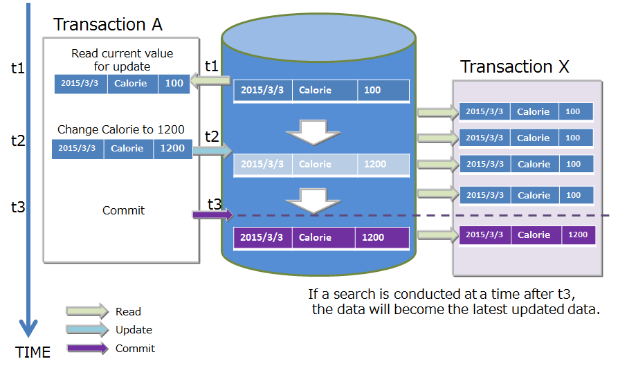
MVCC
4.4.5 Lock
There is a data lock mechanism to maintain the consistency when there are competing container update requests from multiple transactions.
The lock granularity differs depending on the type of container. In addition, the lock range changes depending on the type of operation in the database.
4.4.5.1 Lock granularity
- A timeseries container is a data structure to hold data that is being generated with each passing moment and rarely includes cases in which the data is updated at a specific time.
- Collection data may include cases in which an existing ROW data is updated as it manages data just like a RDB table.
Based on the use case analysis of such a container, the lock granularity (smallest unit) adopted in GridDB is as follows. The lock granularity of a collection which is updated relatively more frequently is a ROW in order to improve the concurrent execution performance.
- Collection: Lock by ROW unit.
-
Timeseries container: Locked by ROW collection
- In a ROW collection, multiple rows are placed in a timeseries container by dividing a block into several data processing units. This data processing unit is known as a row set. It is a data management unit to process a large volume of timeseries containers at a high speed even though the data granularity is coarser than the lock granularity in a collection.
The lock granularity of a collection which is updated randomly more frequently compared to a timeseries container collection adopts a row unit in order to improve the concurrent execution performance.
4.4.5.2 Lock range by database operations
Container operations are not limited to just data registration and deletion but also include schema changes accompanying a change in data structure, index creation to improve speed of access, and other operations. The range of the lock differs between an operation on a specific row of the container and an operation on all rows of the container.
-
Lock equivalent of a container unit
- Index operations (createIndex/dropIndex)
- Container deletion
- Schema change
-
Lock in accordance with the lock granularity
- insert/update/remove
- get(forUpdate)
In a data operation on a row, a lock following the lock granularity is ensured.
If there is competition in securing the lock, the subsequent transaction will be put in standby for securing the lock until the earlier transaction has been completed by a commit or rollback process and the lock is released.
A standby for securing a lock can also be cancelled by a timeout besides completing the execution of the transaction.
4.4.6 Data perpetuation
Data registered or updated in a container or table is perpetuated in the disk or SSD, and protected from data loss when a node failure occurs. There are 2 types of transaction log process, one to synchronize data in a data update and write the updated data sequentially in a transaction log file, and the other is a checkpoint process to store updated data in the memory regularly in the database file on a block basis.
To write to a transaction log, either one of the following settings can be made in the node definition file.
- 0: SYNC
- An integer value of 1 or higher: DELAYED_SYNC
In the "SYNC" mode, log writing is carried out synchronously every time an update transaction is committed or aborted. In the "DELAYED_SYNC" mode, log writing during an update is carried out at a specified delay of several seconds regardless of the update timing. Default value is "1 (DELAYED_SYNC 1 sec)".
When "SYNC" is specified, although the possibility of losing the latest update details when a node failure occurs is lower, the performance is affected in systems that are updated frequently.
On the other hand, if “DELAYED_SYNC" is specified, although the update performance improves, any update details that have not been written in the disk when a node failure occurs will be lost.
If there are 2 or more replicas in a raster configuration, the possibility of losing the latest update details when a node failure occurs is lower even if the mode is set to "DELAYED_SYNC" as the other nodes contain replicas. Consider setting the mode to "DELAYED_SYNC" as well if the update frequency is high and performance is required.
In a checkpoint, the update block is updated in the database file. A checkpoint process operates at the cycle set on a node basis. A checkpoint cycle is set by the parameters in the node definition file. Initial value is 60 sec (1 minute).
By raising the checkpoint execution cycle figure, data perpetuation can be set to be carried out in a time band when there is relatively more time to do so e.g. by perpetuating data to a disk at night and so on. On the other hand, when the cycle is lengthened, the disadvantage is that the number of transaction log files that have to be rolled forward when a node is restarted outside the system process increases, thereby increasing the recovery time.
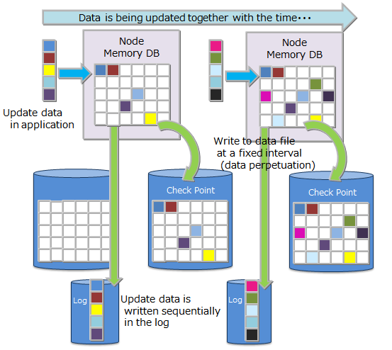
Checkpoint
4.4.7 Timeout process
The timeout details that can be set differ between a NoSQL I/F and a NewSQL I/F.
4.4.7.1 NoSQL I/F timeout
In the NoSQL I/F, 2 types of timeout could be notified to the application developer, Transaction timeout and Failover timeout. The former is related to the processing time limit of a transaction, and the latter is related to the retry time of a recovery process when a failure occurs.
-
TransactionTimeout
The timer is started when access to the container subject to the process begins, and a timeout occurs when the specified time is exceeded.
Transaction timeout is configured to delete lock, and memory from a long-duration update lock (application searches for data in the update mode, and does not delete when the lock is maintained) or a transaction that maintains a large amount of resuts (application does not delete the data when the lock is maintained). Application process is aborted when transaction timeout is triggered.
Besides the node definition file, a transaction timeout can also be specified in the application with a parameter during cluster connection. The specification in the application is prioritized. The default transaction timeout setting is 0 sec. 0 sec means that there is no timeout specified. In order to monitor an extended transaction, set the timeout time to meet the system requirements.
-
FailoverTimeout
Timeout time during an error retry when a client connected to a node constituting a cluster which failed connects to a replacement node. If a new connection point is discovered in the retry process, the client application will not be notified of the error. Default value is 5 minutes. This can also be specified in the application by a parameter during cluster connection. Failover timeout is also used in timeout during initial connection.
Both the transaction timeout and failover timeout can be set when connecting to a cluster using a GridDB object in the Java API or C API. See “GridDB API Reference” (GridDB_API_Reference.html) for details.
4.4.7.2 NewSQL I/F timeout
There are 3 types of timeout as follows:
-
Login (connection) timeout
Timeout for initial connection to the cluster. It can be specified by DriverManager of the application interface. The default value is 300 seconds (5 minutes).
-
Network timeout
Timeout in response between client and cluster. The timeout time is 300 seconds (5 minutes) and can not be changed in the current version.
If the server does not respond for 15 seconds during communication from the client, it will retry, and if there is no response for 5 minutes it will timeout. There is no timeout during long-term query processing.
-
Query timeout
Timeout time can be specified for each query to be executed. The default value is not set to allows long-term query processing. In order to monitor the long-term query, set the timeout time according to the requirements of the system. The setting can be specified by Statement of the application interface.
4.4.8 Replication function
Data replicas are created on a partition basis in accordance with the number of replications set by the user among multiple nodes constituting a cluster.
A process can be continued non-stop even when a node failure occurs by maintaining replicas of the data among scattered nodes. In the client API, when a node failure is detected, the client automatically switches access to another node where the replica is maintained.
The default number of replication is 2, allowing data to be replicated twice when operating in a cluster configuration with multiple nodes.
When there is an update in a container, the owner node (the node having the master replica) among the replicated partitions is updated.
There are 2 ways of subsequently reflecting the updated details from the owner node in the backup node.
-
Asynchronous replication
Replication is carried out without synchronizing with the timing of the asynchronous replication update process. Update performance is better for quasi-synchronous replication but the availability is worse.
-
Quasi-synchronous replication
Although replication is carried out synchronously at the quasi-synchronous replication update process timing, no appointment is made at the end of the replication. Availability is excellent but performance is inferior.
If performance is more important than availability, set the mode to asynchronous replication and if availability is more important, set it to quasi-synchronous replication.
[Memo]
The number of replications is set in the cluster definition file (gs_cluster.json) /cluster/replicationNum. Synchronous settings of the replication are set in the cluster definition file (gs_cluster.json) /transaction/replicationMode.
4.5 Trigger function
A trigger function is an automatic notification function when an operation (add/update or delete) is carried out on the row data of a container. Event notifications can be received without the need to poll and monitor database updates in the application system.
There are 2 ways of notifying the application system.
- Java Messaging Service(JMS)
- REST
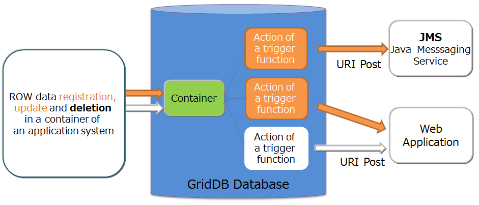
Action of a trigger function
When a trigger occurs, the application can also be notified of the column data in a row data subject to the operation. As to which column data to notify, this is set when the trigger is set in the container. In addition, multiple triggers can also be set in a single container.
The items that can be specified with a trigger setting are as follows.
- Notification event condition (add/update or delete)
- Notification method (JMS or REST)
- Notification column
4.6 Failure process function
In GridDB, recovery for a single point failure is not necessary as replicas of the data are maintained in each node constituting the cluster. The following action is carried out when a failure occurs in GridDB.
- When a failure occurs, the failure node is automatically isolated from the cluster.
- Failover is carried out in the backup node in place of the isolated failure node.
- Partitions are rearranged autonomously as the number of nodes decreases as a result of the failure (replicas are also arranged).
A node that has been recovered from a failure can be incorporated online into a cluster operation. A node can be incorporated into a cluster which has become unstable due to a failure using the gs_joincluster command. As a result of the node incorporation, the partitions will be rearranged autonomously and the node data and load balance will be adjusted.
In this way, although advance recovery preparations are not necessary in a single failure, recovery operations are necessary when operating in a single configuration or when there are multiple overlapping failures in the cluster configuration.
When operating in a cloud environment, even when physical disk failure or processor failure is not intended, there may be multiple failures such as a failure in multiple nodes constituting a cluster, or a database failure in multiple nodes.
4.6.1 Type and treatment of failures
An overview of the failures which occur and the treatment method is shown in the table below.
A node failure refers to a situation in which a node has stopped due to a processor failure or an error in a GridDB server process, while a database failure refers to a situation in which an error has occurred in accessing a database placed in a disk.
| Configuration of GridDB | Type of failure | Action and treatment |
|---|---|---|
| Single configuration | Node failure | Although access from the application is no longer possible, data in a transaction which has completed processing can be recovered simply by restarting the transaction, except when caused by a node failure. Recovery by another node is considered when the node failure is prolonged. |
| Single configuration | Database failure | The database file is recovered from the backup data in order to detect an error in the application. Recovered at the backup point. |
| Cluster configuration | Single node failure | The error is covered up in the application, and the process can continue in nodes with replicas. Recovery operation is not necessary in a node where a failure has occurred. |
| Cluster configuration | Multiple node failure | If both owner/backup partitions of a replica exist in a failure target node , the cluster will operate normally even though the subject partitions cannot be accessed. Except when caused by a node failure, data in a transaction which has completed processing can be recovered simply by restarting the transaction. Recovery by another node is considered when the node failure is prolonged. |
| Cluster configuration | Single database failure | Since data access will continue through another node constituting the cluster when there is a database failure in a single node, the data can be recovered simply by changing the database deployment location to a different disk, and then starting the node again. |
| Cluster configuration | Multiple database failure | A partition that cannot be recovered in a replica needs to be recovered at the point backup data is sampled from the latest backup data. |
4.6.2 Client failover
If a node failure occurs when operating in a cluster configuration, the partitions (containers) placed in the failure node cannot be accessed. At this point, a client failover function to automatically connect to the backup node again and continue the process is activated in the client API. To automatically perform a failover countermeasure in the client API, the application developer does not need to be aware of the error process in the node.
However, due to a network failure or simultaneous failure of multiple nodes, an error may also occur and access to the target application operations may not be possible.
Depending on the data to be accessed, the following points need to be considered in the recovery process after an error occurs.
- For a collection in which the timeseries container or row key is defined, the data can be recovered by executing the failed operation or transaction again.
- For a collection in which the row key is not defined, the failed operation or transaction needs to be executed again after checking the contents of the DB.
[Memo]
In order to simplify the error process in an application, it is recommended that the row key be defined when using a collection. If the data cannot be uniquely identified by a single column value but can be uniquely identified by multiple column values, a column having a value that links the values of the multiple columns is recommended to be set as the row key so that the data can be uniquely identified.
4.6.3 Backup types
It is necessary to collect periodic backups to prepare for data corruption due to database failure or application malfunction. The backup operation method should be selected according to the service level requirements and system resources.
The types of online backup provided by GridDB are as follows. The recovery point varies depending on the type of backup.
| Backup type | Backup actions | Recovery point |
|---|---|---|
| Full backup | A backup of the cluster database currently in use is stored online in node units in the backup directory specified in the node definition file. | Full backup collection point |
| Differential/incremental backup | A backup of the cluster database currently in use is stored online in node units in the backup directory specified in the node definition file. In subsequent backups, only the difference in the update block after the backup is backed up. | Differential/incremental backup collection point |
| Automatic log backup | In addition to backing up the cluster database currently in use which is stored online in node units in the backup directory specified in the node definition file, the transaction log is also automatically picked up at the same timing as the transaction log file writing. The write timing of the transaction log file follows the value of /dataStore/logWriteMode in the node definition file. | Latest transaction update point |
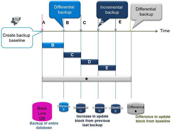
Differential/incremental backup
See “GridDB backup guide” (GridDB_BackupGuide.html) for the backup details and the recovery processes.
4.6.4 Event log function
An event log is a log to record system operating information and messages related to event information e.g. exceptions which occurred internally in a GridDB node etc.
An event log is created with the file name gridstore-%Y%m%d-n.log in the directory shown in the environmental variable GS_LOG (Example: gridstore-20150328-5.log). 22/5000 The file switches at the following timing:
- When the log is written first after the date changes
- When the node is restarted
- When the size of one file exceeds 1MB
The default value of the maximum number of event log files is 30. If it exceeds 30 files, it will be deleted from the old file. The maximum number can be changed with the node definition file.
Output format of event log is as follows.
-
(Date and time) (host name) (thread no.) (log level) (category) [(error trace no.): (error trace no. and name)] (message) < (base64 detailed information: Detailed information for problem analysis in the support service)>
An overview of the event which occurred can be found in the error trace no. and name. In addition, measures to deal with the problems can be searched using the error trace no. in the troubleshooting guide. A output example of an event log is shown below.
2014-11-12T10:35:29.746+0900 TSOL1234 8456 ERROR TRANSACTION_SERVICE [10008:TXN_CLUSTER_NOT_SERVICING] (nd={clientId=2, address=127.0.0.1:52719}, pId=0, eventType=CONNECT, stmtId=1) <Z3JpZF9zdG9yZS9zZXJ2ZXIvdHJhbnNhY3Rpb25fc2VydmljZS5jcHAgQ29ubmVjdEhhbmRsZXI6OmhhbmRsZUVycm9yIGxpbmU9MTg2MSA6IGJ5IERlbnlFeGNlcHRpb24gZ3JpZF9zdG9yZS9zZXJ2ZXIvdHJhbnNhY3Rpb25fc2VydmljZS5jcHAgU3RhdGVtZW50SGFuZGxlcjo6Y2hlY2tFeGVjdXRhYmxlIGxpbmU9NjExIGNvZGU9MTAwMDg=>
The event log output level can be changed online by using the gs_logconf command. When analyzing details of trouble information, change it online. However, online changes are temporary memory changes. Therefore, in order to make it permanent such as setting valid at restart of the node, it is necessary to change the trace item of the node definition file of each node constituting the cluster.
The current setting can be displayed with the gs_logconf command.
$ gs_logconf -u admin/admin
{
    "levels": {
        "CHECKPOINT_FILE": "ERROR",
        "CHECKPOINT_SERVICE": "INFO",
        "CHUNK_MANAGER": "ERROR",
        "CHUNK_MANAGER_IODETAIL": "ERROR",
        "CLUSTER_OPERATION": "INFO",
        "CLUSTER_SERVICE": "ERROR",
        "COLLECTION": "ERROR",
        "DATA_STORE": "ERROR",
        "DEFAULT": "ERROR",
        "EVENT_ENGINE": "WARNING",
        "IO_MONITOR": "WARNING",
        "LOG_MANAGER": "WARNING",
        "MAIN": "WARNING",
        "MESSAGE_LOG_TEST": "ERROR",
        "OBJECT_MANAGER": "ERROR",
        "RECOVERY_MANAGER": "INFO",
        "REPLICATION_TIMEOUT": "WARNING",
        "SESSION_TIMEOUT": "WARNING",
        "SYNC_SERVICE": "ERROR",
        "SYSTEM": "UNKNOWN",
        "SYSTEM_SERVICE": "INFO",
        "TIME_SERIES": "ERROR",
        "TRANSACTION_MANAGER": "ERROR",
        "TRANSACTION_SERVICE": "ERROR",
        "TRANSACTION_TIMEOUT": "WARNING",
        "TRIGGER_SERVICE": "ERROR"
    }
}
4.7 Data access
To access GridDB data, there is a need to develop an application using NoSQL I/F or NewSQL I/F (GridDB AE/VE only). Data can be accessed simply by connecting to the cluster database of GridDB without having to take into account position information on where the container or table is located in the cluster database. The application system does not need to consider which node constituting the cluster the container is placed in.
In the GridDB API, when connecting to a cluster database initially, placement hint information of the container is retained (cached) on the client end together with the node information (partition).
Communication overheads are kept to a minimum as the node maintaining the container is connected and processed directly without having to access the cluster to search for nodes that have been placed every time the container used by the application is switched.
Although the container placement changes dynamically due to the rebalancing process in GridDB, the position of the container is transmitted as the client cache is updated regularly. For example, even when there is a node mishit during access from a client due to a failure or a discrepancy between the regular update timing and re-balancing timing, relocated information is automatically acquired to continue with the process.
4.7.1 TQL and SQL
TQL and SQL-92 compliant SQL (GridDB AE/VE only) are supported as database access languages.
-
What is TQL?
A simplified SQL prepared for GridDB SE. The support range is limited to functions such as search, aggregation, etc., using a container as a unit. TQL is employed by using the client API (Java, C language) of GridDB SE.
The TQL is adequate for the search in the case of a small container and a small number of hits. For that case, the response is faster than SQL. The number of hits can be suppressed by the LIMIT clause of TQL.
For the search of a large amount of data, SQL is recommended.
TQL is available for the containers and paritioned tables created by operations through the NewSQL interface. The followings are the limitations of TQL for the partitioned tables.
- Filtering data by the WHERE clause is available. But aggregate functions, timeseries data selection or interpolation, min or max function and ORDER BY clause, etc. are not available.
- It is not possible to apply the update lock.
-
What is SQL?
Standardization of the language specifications is carried out in ISO to support the interface for defining and performing data operations in conformance with SQL-92 in GridDB. SQL can be used in NewSQL I/F.
SQL is also available for the containers created by operations through the NoSQL interface.
See “GridDB API Reference” (GridDB_API_Reference.html) for details on TQL, and “GridDB AE SQL Reference” (GridDB_AE_SQL_Reference.pdf) for details on SQL.
4.7.2 NoSQL I/F characteristic functions
An interface to quickly process event information that occurs occasionally is available in NoSQL I/F.
When a large volume of events is sent to the database server every time an event occurs, the load on the network increases and system throughput does not increase. Significant impact will appear especially when the communication line bandwidth is narrow. Multi-processing is available in NoSQL I/F to process multiple row registrations for multiple containers and multiple inquiries (TQL) to multiple containers with a single request. The overall throughput of the system rises as the database server is not accessed frequently.
An example is given below.
-
Multiput
A container is prepared for each sensor name as a process to register event information from multiple sensors in the database. The sensor name and row array of the timeseries event of the sensor are created and a list (map) summarizing the data for multiple sensors is created. This list data is registered in the GridDB database each time the API is invoked.
In the API of a multi- registration process, the communication process is optimized by consolidating requests for 1 or more containers to a node in GridDB formed by multiple clusters. In addition, multi-registrations are processed quickly without performing MVCC when executing a transaction.
In a multiput, transactions are committed automatically. Data is confirmed on a single case basis.
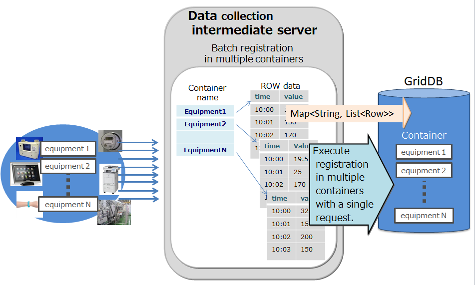
Multiput
-
Multi-query (fetchAll)
Instead of executing multiple queries to a sensor, these can be executed in a single query by consolidating event information of the sensor. For example, this is most suitable for acquiring aggregate results such as the daily maximum, minimum and average values of data acquired from a sensor, or data of a row set having the maximum or minimum value, or data of a row set meeting the specified condition.
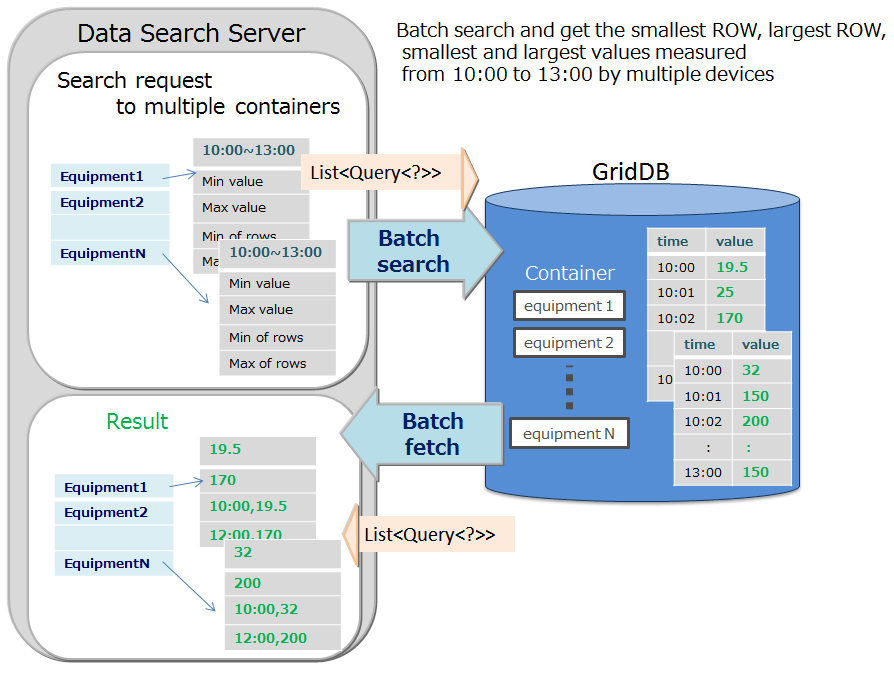
fetchAll
-
Multiget
Instead of executing multiple queries to a sensor, these can be executed in a single query by consolidating event information of the sensor. For example, this is most suitable for acquiring aggregate results such as the daily maximum, minimum and average values of data acquired from a sensor, or data of a row set having the maximum or minimum value, or data of a row set meeting the specified condition.
In a RowKeyPredicate object, the acquisition condition is set in either one of the 2 formats below.
- Specify the acquisition range
- Specified individual value
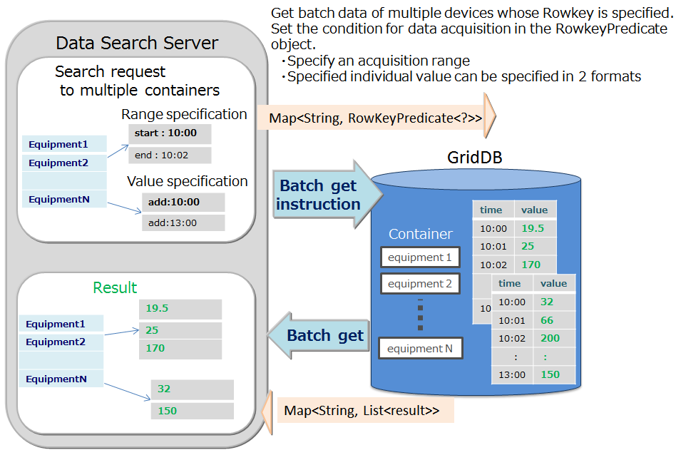
Multiget
4.8 Operating function
Explain the outline of GridDB operation function. See "GridDB operation control guide" (GridDB_OperationGuide.html) for details.
4.8.1 Service
GridDB service is automatically performed during OS start-up to start a node or cluster.
GridDB service is enabled after installing with RPM. Since the service is enabled, the GridDB server is started at the same time the OS starts up, and the server is stopped when the OS is stopped.
When you use an interface that integrates middleware and application operation including OS monitoring and database software operation, consideration of dependency with other middleware such as whether to use service or operating commands for GridDB operation is necessary.
See "GridDB operation control guide" (GridDB_OperationGuide.html) for parameters of the service.
If service is not used, disable the service as follows:
# /sbin/chkconfig gridstore off
4.8.2 Operating commands
The following commands are available in GridDB.
| Type | Command | Function |
|---|---|---|
| Start/stop node | gs_startnode | Start a node |
| gs_stopnode | Stop a node | |
| Cluster management | gs_joincluster | Join to cluster configuration |
| gs_leavecluster | Leave from cluster configuration | |
| gs_stopcluster | Stop a cluster | |
| gs_config | Get cluster configuration data | |
| gs_stat | Get cluster data | |
| gs_appendcluster | Add a node to a cluster | |
| gs_failovercluster | Do manual failover of a cluster | |
| gs_partition | Get partition data | |
| gs_loadbalance | Set autonomous data redistribution | |
| User management | gs_adduser | Add an administrator user |
| gs_deluser | Delete an administrator user | |
| gs_passwd | Change a password of an administrator user | |
| Log data | gs_logs | Display recent event logs |
| gs_logconf | Display and change the event log output level | |
| Backup/restoration | gs_backup | Collect backup data |
| gs_backuplist | Display backup data list | |
| gs_restore | Restore a backup data | |
| Import/export | gs_import | Import exported containers and database on the disk |
| gs_export | Export containers and database as CSV or ZIP format to the disk | |
| Maintenance | gs_paramconf | Display and change parameters |
4.8.3 Integrated operation control GUI (gs_admin)
The integrated operation control GUI (hereinafter referred to gs_admin) is a Web application that integrates GridDB cluster operation functions. Gs_admin has an intuitive UI, it is possible to grasp the operation information of the cluster on one screen (dashboard screen), start and stop operation to individual nodes constituting the cluster, check performance information, etc.
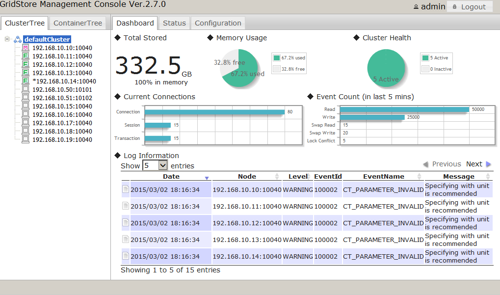
Gs_admin dashboard screen
Gs_admin also supports the following functions to support development, so it can be used effectively in the development stage of the system.
- Create and drop database, manage general user
- Create, drop and search container
- Create and drop index and trigger
- Execute TQL/SQL statement to container
4.8.4 Cluster operation control command interpreter (gs_sh)
The cluster operation control command interpreter (hereinafter referred to gs_sh) is a command line interface tool to manage GridDB cluster operations and data operations. While operating commands provide operation on a per-node basis, gs_sh provides interfaces for processing on a per-cluster basis. In addition to user management operations, it also provides data manipulation such as creating databases, containers and tables, and searching by TQL or SQL.
There are two types of start modes in gs_sh.
- Interactive mode: specify subcommand interactively to execute processing
- Batch mode: Execute a script file containing a series of operations with subcommands
Use of batch script enables automation of operation verification at development and labor saving of system construction
Gs_sh has its own variable definition function, and operations on nodes and clusters can also be executed with instructions to the operation target whose variables are defined in advance.
// Interactive mode: start gs_sh and execute subcommand "version"
$ gs_sh
gs> version

// Batch mode: execute a script file specified as an argument
$ gs_sh test.gsh
The following subcommands are available in gs_sh.
| Type | Subcommand | Function |
|---|---|---|
| Start/stop node | startnode | Start nodes. Starting all nodes of the cluster and waiting for startup completion are possible. |
| stopnode | Stop nodes. Stopping all nodes of the cluster is possible. | |
| Cluster management | joincluster | Attach a node individually to a cluster. |
| leavecluster | Detach a node individually from a cluster. | |
| stopcluster | Detach all of the currently attached nodes from a cluster, together at once. | |
| config | Display the cluster configuration data. | |
| configcluster | Display the cluster status data. | |
| appendcluster | Add an undefined node to a pre-defined cluster. | |
| Connection | connect | Connect to a GridDB cluster. For GridDB AE/VE, connect with both NoSQL I/F and NewSQL I/F, and can be used both TQL and SQL. |
| disconnect | Disconnect from a GridDB cluster. | |
| Database management | createdatabase | Create a database. |
| dropdatabase | Delete a database. | |
| getcurrentdatabase | Display the current database name. | |
| showdatabase | Display the database list and access rights data. | |
| General user management | createuser | Create a general user. |
| dropuser | Delete a general user. | |
| setpassword | Change the password of a general user. | |
| showuser | Display the user data. | |
| Access control | grant | Grant access rights for a user to a database. |
| revoke | Revoke access rights for a user from a database. | |
| Container operation | createcontainer | Create a container from the container data file. |
| createcollection | Create a collection of simple schema. | |
| createtimeseries | Create a timeseries container of simple schema. | |
| dropcontainer | Delete a container. | |
| showcontainer | Display the container data. | |
| Table operation (GridDB AE/VE) | showtable | Display the table data. |
| Index operation | createindex | Create an index in the specified column. |
| dropindex | Delete an index in the specified column. | |
| Trigger operation | droptrigger | Delete a trigger from a container. |
| showtrigger | Show trigger data of a container. | |
| TQL/SQL | tql | Execute a TQL and retain the search results from a container. |
| get/getnoprint | Get the search results. | |
| getcsv | Get the search results and save them in a file in the CSV format. | |
| tqlexplain | Execute the specified TQL and display the execution plan and actual measurement values such as the number of cases processed etc. | |
| sql (GridDB AE/VE) | Execute an SQL and retain the search results from a table or container. | |
| Log data | logs | The following command displays the log of the specified node. |
| logconf | Display and change the log settings. |
4.8.5 Performance and statistical information
GridDB performance and statistical information can be checked in GridDB using the operating command gs_stat. gs_stat represents information common in the cluster and performance and statistical information unique to the nodes.
Among the outputs of the gs_stat command, the performance structure is an output that is related to the performance and statistical information.
-bash-4.1$ gs_stat -u admin/admin -s 192.168.0.1:10040
{
    :
    "performance": {
        "batchFree": 0,
        "checkpointFileSize": 65536,
        "checkpointFileUsageRate": 0,
        "checkpointMemory": 2031616,
        "checkpointMemoryLimit": 1073741824,
        "checkpointWriteSize": 0,
        "checkpointWriteTime": 0,
        "currentTime": 1428024628904,
        "numConnection": 0,
        "numTxn": 0,
        "peakProcessMemory": 42270720,
        "processMemory": 42270720,
        "recoveryReadSize": 65536,
        "recoveryReadTime": 0,
        "storeDetail": {
            "batchFreeMapData": {
                "storeMemory": 0,
                "storeUse": 0,
                "swapRead": 0,
                "swapWrite": 0
            },
            "batchFreeRowData": {
                "storeMemory": 0,
                "storeUse": 0,
                "swapRead": 0,
                "swapWrite": 0
            },
            "mapData": {
                "storeMemory": 0,
                "storeUse": 0,
                "swapRead": 0,
                "swapWrite": 0
            },
            "metaData": {
                "storeMemory": 0,
                "storeUse": 0,
                "swapRead": 0,
                "swapWrite": 0
            },
            "rowData": {
                "storeMemory": 0,
                "storeUse": 0,
                "swapRead": 0,
                "swapWrite": 0
            }
        },
        "storeMemory": 0,
        "storeMemoryLimit": 1073741824,
        "storeTotalUse": 0,
        "swapRead": 0,
        "swapReadSize": 0,
        "swapReadTime": 0,
        "swapWrite": 0,
        "swapWriteSize": 0,
        "swapWriteTime": 0,
        "syncReadSize": 0,
        "syncReadTime": 0,
        "totalLockConflictCount": 0,
        "totalReadOperation": 0,
        "totalRowRead": 0,
        "totalRowWrite": 0,
        "totalWriteOperation": 0
    },
    :
}
Information related to performance and statistical information is explained below. The description of the storeDetail structure is omitted as this is internal debugging information.
-
The type is shown below.
- CC: Current value of all cluster
- c: Current value of specified node
- CS: Cumulative value after service starts for all clusters
- s: Cumulative value after service starts for all nodes
- CP: Peak value after service starts for all clusters
- p: Peak value after service starts for all nodes
-
Check the event figure to be monitored, and show the items that ought to be reviewed in continuing with operations.
Output parameters Type Description Event to be monitored checkpointFileSize c Checkpoint file size (byte) checkpointFileUsageRate c Checkpoint file usage rate checkpointMemory c Checkpoint memory size for checkpoint use (byte) checkpointMemoryLimit c CheckpointMemoryLimit setting for checkpoint use (byte) checkpointWriteSize s Checkpoint process CP file write size (byte) checkpointWriteTime s Checkpoint process CP file write time checkpointFileAllocateSize c Total size of allocated blocks in checkpoint files (byte) currentTime c Current time numConnection c Current no. of connections. Number of connections used in the transaction process, not including the number of connections used in the cluster process. Value is equal to the no. of clients + no. of replicas \* no. of partitions retained. If the no. of connections is insufficient in monitoring the log, review the connectionLimit value of the node configuration. numSession c Current no. of sessions numTxn c Current no. of transactions peakProcessMemory p Peak value of the memory used in the GridDB server, including the storememory value which is the maximum memory size (byte) used in the process If the peakProcessMemory or processMemory is larger than the installed memory of the node and an OS Swap occurs, additional memory or a temporary drop in the value of the storeMemoryLimit needs to be considered. processMemory c Memory space used by a process (byte) recoveryReadSize s Checkpoint file size read by the recovery process (byte) recoveryReadTime s Checkpoint file time read by the recovery process (byte) storeMemory c Memory space used in an in-memory database (byte) storeMemoryLimit c Memory space limit used in an in-memory database (byte) storeTotalUse c Full data capacity (byte) retained by the nodes, including the data capacity in the database file swapRead s Swap read count swapReadSize s Swap process file read size (byte) swapReadTime s Swap process file read time swapWrite s Swap write count swapWriteSize s Swap process file write size (byte) swapWriteTime s Swap process file write time syncReadSize s Synchronization process CP file read size (byte) syncReadTime s Synchronization process CP file read time totalLockConflictCount s Row lock competing count totalReadOperation s Search process count totalRowRead s Insert and update process count totalRowWrite s Row reading count totalWriteOperation s Row writing count
4.8.6 Rolling upgrade
The upgrade of nodes while the cluster is running is possible by the rolling upgrade. By operating one by one to leave a node from the cluster, upgrading GridDB on the node and join the node to the cluster again, GridDB on all nodes are replaced to a newer version.
-
Make a plan for the operations of rolling upgrade in advance
Estimate the time of the operations. The operations for a node are as follows. Estimate the time of the following operations and calculate the time for all the nodes. The estimated time is a few minutes for the operations other than the start-up of a node (recovery).
- Leave cluster
- Stop node
- Installation of GridDB
- Start-up node (recovery)
- Join cluster
When there are many data updates before leaving the cluster or during the rolling upgrade, the recovery may take longer than usual.
-
Disable autonomous data redistribution
In the rolling upgrade, after each node leaves the cluster, it rejoins the cluster soon. By disabling autonomous data redistribution, redundant redistributions can be eliminated and the load of the processing and network communication can be reduced.
By executing the gs_loadbalance command with the --cluster option, the autonomous data redistribution on all the nodes of the cluster is disabled.
Example)
$ gs_loadbalance -u admin/admin --off --cluster
-
Upgrade the nodes other than the master node
Perform the following operations on each node. Login the node and do the operations. From starting these operations and until finishing step 5, the operations of SQL cause an error.
a. Check the role of each node
Execute the gs_stat command. Do the step b. and the subsequence operations on the nodes which are display '"clusterStatus": "FOLLOWER"'.
Example)
$ gs_stat -u admin/admin
・・・
"clusterStatus": "FOLLOWER"
b. Leave the cluster (gs_leavecluster)
Example)
$ gs_leavecluster -u admin/admin --force
c. Stop the node (gs_stopnode)
Example)
$ gs_stopnode -u admin/admin
d. Upgrade GridDB
The process of upgrading is different for each of the version. See the quick start guide about the operations.
e. Start-up the node
Example)
$ gs_startnode -u admin/admin
f. Disable autonomous data redistribution
The --cluster option is not needed because of the operation on single node.
Example)
$ gs_loadbalance -u admin/admin --off
g. Join the node to the cluster (gs_join)
Example) Cluster name: mycluster, The number of nodes in the cluster: 5
$ gs_joincluster -u admin/admin -c mycluster -n 5
-
Upgrade the master node
a. Check the role of each node
Execute the gs_stat command. Do the step b. and the subsequence operations on the nodes which are display '"clusterStatus": "MASTER"'.
Example)
$ gs_stat -u admin/admin
・・・
"clusterStatus": "MASTER"
b. Leave the cluster (gs_leavecluster) The cluster stops temporarily (for about 1 minutes) by this operation
c. Stop the node (gs_stopnode)
d. Upgrade GridDB
e. Start-up the node
f. Disable autonomous data redistribution
g. Join the node to the cluster (gs_joincluster)
- Check that all nodes are the new version (gs_stat)
-
Enable autonomous data redistribution on all nodes in the cluster (gs_loadbalance)
$ gs_loadbalance -u admin/admin --on --cluster
[Memo]
- The rolling upgrade can be used for version 4.0 or later.
-
The rolling upgrade can not be performed when the current major version and the replaced major version of the cluster are different.
Example) When the current version is V4.0 and the version to be replaced is V5.0, the rolling upgrade cannot be performed because the major versions are different.
- The replaced version is required to be newer than the current version.
[Notes]
- When different versions are mixed in a cluster by the rolling upgrade, an error may occur in a SQL search. The limitations will be explained in each version's Readme file, so please see the Readme file for the limitations. (The SQL search is retried repeatedly in the failover time. In the meantime, if the rolling upgrade is finished, the error does not occur on the client.)
- When the master node is replaced, the cluster stops temporarily (about 1 minute). For the processing that can be failed over (NoSQL interface and SQL search), if the cluster restarts in the failover time, no error occurs on the client.
- When there are many data updates during a rolling upgrade, the synchronization of data takes time. It is recommended to perform the rolling upgrade during the hours when there are fewer data updates.
5 Parameters
Describes the parameters to control the operations in GridDB. In the GridDB parameters, there is a node definition file to configure settings such as the setting information and usable resources etc., and a cluster definition file to configure operational settings of a cluster. Explains the meanings of the item names in the definition file and the settings and parameters in the initial state.
The unit of the setting is set as shown below.
- The byte size can be specified in the following units: TB, GB, MB, KB, B, T, G, M, K, or lowercase notations of these units Unit cannot be omitted unless otherwise stated.
- Time can be specified in the following units: h, min, s, ms. Unit cannot be omitted unless otherwise stated.
5.1 Cluster definition file(gs_cluster.json)
The same setting in the cluster definition file needs to be made in all the nodes constituting the cluster. As the partitionNum and storeBlockSize parameters are important parameters to determine the database structure, they cannot be changed when GridDB is started after the system is built.
The cluster name is a parameter that must be set from V2.7 onwards.
The meanings of the various settings in the cluster definition file are explained below.
By adding an item name, items that are not included in the initial state can be recognized by the system. Indicate whether the parameter can be changed and the change timing in the change field.
- Disallowed: Node cannot be changed once it has been started. The database needs to be initialized if you want to change the setting.
- Restart: Parameter can be changed by restarting all the nodes constituting the cluster.
-
Online: Parameters that are currently in operation online can be changed. However, the contents in the definition file need to be manual amended as the change details will not be perpetuated.
Configuration of GridDB Default Meaning of parameters and limitation values Change /notificationAddress 239.0.0.1 Standard setting of a multi-cast address. This setting will become valid if a parameter with the same cluster, transaction name is omitted. If a different value is set, the address of the individual setting is valid. Restart /dataStore/partitionNum 128 Specify a common multiple that will allow the number of partitions to be divided and placed by the number of constituting clusters Integer: Specify an integer that is 1 or higher and 10000 or lower. Disallowed /dataStore/storeBlockSize 64KB Specify the disk I/O size. Either 64KB or 1MB can be specified. Assume and set the data occurrence frequency. Cannot be changed after server is started. Disallowed /cluster/clusterName - Specify the name for identifying a cluster. Mandatory input parameter. Restart /cluster/replicationNum 2 No. of replicas. Partition is doubled if the no. of replicas is 2. Restart /cluster/notificationAddress 239.0.0.1 Multi-cast address for cluster configuration Restart /cluster/notificationPort 20000 Specify a value within a specifiable range as a multi-cast port no. for a cluster configuration. Restart /cluster/notificationInterval 5s Specify a multi-cast period of 1s or more, or 2^31s or less for the cluster configuration. Restart /cluster/heartbeatInterval 5s Specify a check period (heart beat period) of 1s or more, and less than 2^31s, to check the node survival among clusters. Restart /cluster/loadbalanceCheckInterval 180s In order to adjust the load balance among nodes constituting the cluster, specify a data sampling period of 1s or more, and less than 2^31s, with the unit omitted when determining whether to implement the balancing process or not. Restart /cluster/notificationMember - Specify the address list when using the fixed list method as the cluster configuration method. Restart /cluster/notificationProvider/url - Specify the URL of the address provider when using the provider method as the cluster configuration method. Restart /cluster/notificationProvider/updateInterval 5s Specify the interval to get the list from the address provider. Specify a value that is 1s or higher and less than 2^31s. Restart /sync/timeoutInterval 30s Timeout time during data synchronization among clusters If a timeout occurs, the system load may be high, or a failure may have occurred. Specify a value that is 1s or higher and less than 2^31s. Restart /transaction/notificationAddress 239.0.0.1 Multi-cast address that a client connects to initially. Master node is notified in the client. Restart /transaction/notificationPort 31999 Multi-cast port that a client connects to initially. Specify a value within a specifiable range as a multi-cast port no. Restart /transaction/notificationInterval 5s Multi-cast period for a master to notify its clients. Specify a value that is 1s or higher and less than 2^31s. Restart /transaction/replicationMode 0 Specify the data synchronization (replication) method when updating the data in a transaction. Specify a string or integer, "ASYNC"or 0 (non-synchronous), "SEMISYNC"or 1 (quasi-synchronous). Restart /transaction/replicationTimeoutInterval 10s Specify the timeout time for communications among nodes when synchronizing data in a quasi-synchronous replication transaction. Specify a value that is 1s or higher and less than 2^31s. Restart /sql/notificationAddress 239.0.0.1 Multi-cast address when the JDBC/ODBC client is connected initially. Master node is notified in the client. Restart /sql/notificationPort 41999 Multi-cast port when the JDBC/ODBC client is connected initially. Specify a value within a specifiable range as a multi-cast port no. Restart /sql/notificationInterval 5s Multi-cast period for a master to notify its JDBC/ODBC clients. Specify a value that is 1s or higher and less than 2^31s. Restart
5.2 Node definition file (gs_node.json)
Default setting of the resources in nodes constituting a cluster. In an online operation, there are also parameters whose values can be changed online from the resource, access frequency, etc., that have been laid out. Conversely, note that there are also values (concurrency) that cannot be changed once set.
The meanings of the various settings in the node definition file are explained below.
By adding an item name, items that are not included in the initial state can be recognized by the system. Indicate whether the parameter can be changed and the change timing in the change field.
- Disallowed: Node cannot be changed once it has been started. The database needs to be initialized if you want to change the setting.
- Restart: Parameter can be changed by restarting all the nodes constituting the cluster.
- Online: Parameters that are currently in operation online can be changed. However, the contents in the definition file need to be manual amended as the change details will not be perpetuated.
Specify the directory by specifying the full path or a relative path from the GS_HOME environmental variable. For relative path, the initial directory of GS_HOME serves as a reference point. Initial configuration directory of GS_HOME is /var/lib/gridstore.
| Configuration of GridDB | Default | Meaning of parameters and limitation values | Change |
|---|---|---|---|
| /serviceAddress | - | Set the initial value of each cluster, transaction, sync service address. The initial value of each service address can be set by setting this address only without having to set the addresses of the 3 items. | Restart |
| /dataStore/dbPath | data | The deployment directory of the database file is specified by the full path or a relative path | Restart |
| /dataStore/backupPath | backup | Specify the backup file deployment directory path. | Restart |
| /dataStore/syncTempPath | sync | Data sync temporary file directory | Restart |
| /dataStore/storeMemoryLimit | 1024MB | Upper memory limit for data management | Online |
| /dataStore/concurrency | 4 | Concurrency | Disallowed |
| /dataStore/logWriteMode | 1 | If the log writing mode period is -1 or 0, log writing is performed at the end of the transaction. If it is 1 or more and less than 2^31, log writing is performed at a period specified in seconds | Restart |
| /dataStore/persistencyMode | 1(NORMAL) | In the perpetuation mode, the period that the update log file is maintained during a data update is specified. Specify either 1 (NORMAL) or 2 (RETAINING_ALL_LOGS). For "NORMAL", a transaction log file which is no longer required will be deleted by the checkpoint. For "RETAINING_ALL_LOGS", all transaction log files are retained. Default value is "1 (NORMAL)". | Restart |
| /dataStore/storeWarmStart | false(invalid) | Specify whether to save in-memory up to the upper limit of the chunk memory during a restart. | Restart |
| /dataStore/affinityGroupSize | 4 | Number of affinity groups | Restart |
| /dataStore/storeCompressionMode | NO_COMPRESSION | Data block compression mode | Restart |
| /checkpoint/checkpointInterval | 60s | Checkpoint process execution period to perpetuate a data update block in the memory | Restart |
| /checkpoint/checkpointMemoryLimit | 1024MB | Upper limit of special checkpoint write memory* Pool the required memory space up to the upper limit when there is a update transaction in the checkpoint. | Online |
| /checkpoint/useParallelMode | false(invalid) | Specify whether to execute the checkpoint concurrently. *The no. of concurrent threads is the same as the concurrency. | Restart |
| /checkpoint/checkpointCopyInterval | 100ms | Output process interval when outputting a block with added or updated data to a disk in a checkpoint process. | Restart |
| /cluster/serviceAddress | Follow the “/serviceAddress” | Standby address for cluster configuration | Restart |
| /cluster/servicePort | 10010 | Standby port for cluster configuration | Restart |
| /sync/serviceAddress | Follow the “/serviceAddress” | Specify the reception address for data synchronization among the clusters. | Restart |
| /sync/servicePort | 10020 | Standby port for data synchronization | Restart |
| /system/serviceAddress | Follow the “/serviceAddress” | Standby address for operation commands | Restart |
| /system/servicePort | 10040 | Standby port for operation commands | Restart |
| /system/eventLogPath | log | Event log file deployment directory path | Restart |
| /transaction/serviceAddress | Follow the “/serviceAddress” | Standby address for transaction process | Restart |
| /transaction/servicePort | 10001 | Standby port for transaction process | Restart |
| /transaction/connectionLimit | 5000 | Upper limit of the no. of transaction process connections | Restart |
| /transaction/transactionTimeoutLimit | 300s | Transaction timeout upper limit. | Restart |
| /sql/serviceAddress | Follow the “/serviceAddress” | Standby address for New SQL access process | Restart |
| /sql/servicePort | 20001 | Standby port for New SQL access process | Restart |
| /sql/storeSwapFilePath | swap | SQL intermediate store swap file directory | Restart |
| /sql/storeSwapSyncSize | 1024MB | SQL intermediate store swap file and cache size | Restart |
| /sql/storeMemoryLimit | 1024MB | Upper memory limit for intermediate data held in memory by SQL processing. | Restart |
| /sql/workMemoryLimit | 128MB | Upper memory limit for operators in SQL processing | Restart |
| /sql/workCacheMemory | 128MB | Upper size limit for cache without being released after use of work memory. | Restart |
| /sql/connectionLimit | 5000 | Upper limit of the no. of connections processed for New SQL access | Restart |
| /sql/concurrency | 5 | No. of simultaneous execution threads | Restart |
| /trace/fileCount | 30 | Upper file count limit for event log files. | Restart |
6 Terminology
Describes the terms used in GridDB in a list.
| Terms | Meaning |
|---|---|
| Node | Refers to the individual server process to perform data management in GridDB. |
| Cluster | Refers to a single or a set of multiple nodes to perform data management together. |
| Master node | Node to perform a cluster management process. |
| Follower node | A node participating in a cluster except the master node. |
| Designated node count | Refers to the number of nodes constituting a GridDB cluster. When starting GridDB for the first time, the number is used as a threshold value for the cluster to be valid. (Cluster service is started when the number of nodes constituting a cluster joins the cluster.) |
| Active node count | Number of nodes currently in operation that have been incorporated into the cluster among the nodes constituting the GridDB cluster. |
| Block | A block is a data unit for data perpetuation in a disk (hereinafter referred to a checkpoint) and is the smallest physical data management unit in GridDB. Multiple container data is placed in a block. Before initial startup of GridDB, a size of either 64 KB or 1 MB can be selected for the block size to be set up in the definition file (cluster definition file). Specify 64 KB if the installed memory of the system is low, or if the frequency of data increase is low. |
| Partition | Data management unit to arrange a container. Smallest data placement unit between clusters and data movement and replication unit for adjusting the load balance between nodes (rebalance) and for managing the data multiplexing (replica) in case of a failure. |
| Partition group | A group summarizing multiple partitions which is equivalent to the data file in the file system when the data is perpetuated in a disk. 1 checkpoint file corresponds to 1 partition group. Partition groups are created according to concurrency (/dataStore/concurrency) figure in the node definition file. |
| Row | Refers to 1 row of data registered in a container or table. Multiple rows are registered in a container or table. Columns of multiple data type are created in a row. |
| Container (table) | Data structure serving as an I/F with the user. Container to manage a set of rows. It is called a container when operating with NoSQL I/F, and a table when operating with NewSQL I/F. 2 data types exist, collection (table) and timeseries container (timeseries table). |
| Collection (table) | One type of container (table) to manage rows having a general key. |
| Timeseries container (timeseries table) | One type of container (table) to manage rows having a timeseries key. Possesses a special function to handle timeseries data. |
| Database file | A perpetuated file group to write data saved in a node that constitutes a cluster into a disk or SSD. A database file is a generic term to describe the transaction log file that is saved every time the GridDB database is updated and the checkpoint file that is written regularly by the database in the memory. |
| Checkpoint file | A partition group is a file written into a disk. Update information is reflected in the memory by a cycle of the node definition file (/checkpoint/checkpointInterval). |
| Transaction log file | Transaction update information is save sequentially as a log. |
| LSN (Log Sequence Number) | Shows the update log sequence no. when updating in the transaction assigned to each partition. The master node of a cluster configuration contains the maximum LSN (MAXLSN) of all the partitions maintained by each node. |
| Replica | Refers to the multiplexing placement of partitions in multiple nodes. A replica may be an owner replica which is master data to be updated or a backup replica used for reference purposes. |
| Owner node | A node that can update a container in a partition. A node that records the container serving as a master among the replicated containers. |
| Backup node | A node that records the container serving as a replica among the replicated containers. |
| Definition file | There are 2 types of definition file, a parameter file (gs_cluster.json: hereinafter referred to a cluster definition file) when composing a cluster, and a parameter file (gs_node.json: hereinafter referred to a node definition file) to set the operations and resources of the node in the cluster. In addition, there is also a user definition file for GridDB administrator users. |
| Event log file | The operating log of the GridDB server is saved. Messages such as errors, warnings, etc. are saved. |
| OS user (gsadm) | A user known as gsadm is created during GridDB installation and who has the right to execute operating functions in GridDB. |
| Administrator user | An administrator user is a GridDB use prepared to perform operations in GridDB. |
| General user | A user used in the application system. |
| User definition file | File in which an administrator user is registered. During initial installation, 2 administrators, system and admin, are registered. |
| Cluster database | General term for all databases that can be accessed in a GridDB cluster system. |
| Database | Theoretical data management unit created in a cluster database. A public database is created in a cluster database by default. Data separation can be realized for each user by creating a new database and giving a general user the right to use it. |
| Full backup | A backup of the cluster database currently in use is stored online in the backup directory specified in the node definition file. |
| Incremental backup (Cumulative/Differential backup) | A backup of the cluster database currently in use is stored online in the backup directory specified in the node definition file. In subsequent backups, only the difference in the update block after the backup is backed up. |
| Auto log backup | In addition to backing up the cluster database currently in use in the specified directory online, the transaction log is also automatically picked up at the same timing as the transaction log file writing. The write timing of the transaction log file follows the value of /dataStore/logWriteMode in the node definition file. |
| Failover | When a failure occurs in a cluster currently in operation, the structure allows the backup node to automatically take over the function and continue with the processing. |
| Client failover | When a failure occurs in a cluster currently in operation, the structure allows the backup node to be automatically re-connected to continue with the processing as a retry process when a failure occurs in the API on the client side. |
| Table partitioning | Function to access a huge table quickly by allowing concurrent execution by processors of multiple nodes, and the memory of multiple nodes to be used effectively by distributing the placement of a large amount of table data with multiple data registrations in multiple nodes. |
| Data partition | General name of data storage divided by table partitioning. Multiple data partitions are created for a table by table partitioing. Data partitions are distributed to the nodes like normal containers. The number of data partitions and the range of data stored in each data partition are depending on the type of table partitioning (hash, interval or interval-hash). |
| Data affinity | A function to raise the memory hit rate by placing highly correlated data in a container in the same block and localizing data access. |
| Node affinity | A function to reduce the network load when accessing data by placing highly correlated containers and tables in the same node. |
7 System limiting values
7.1 Limitations on numerical value
| Block size | 64KB | 1MB |
|---|---|---|
| STRING/GEOMETRY data size | 31KB | 128KB |
| BLOB data size | 1GB - 1Byte | 1GB - 1Byte |
| Array length | 4000 | 65000 |
| No. of columns | 1024 | 1024 |
| No. of columns subject to linear complementary compression | 100 | 100 |
| Size of container name / index name | Approx. 16KB | Approx. 128KB |
| Size of column | 256Byte | 256Byte |
| Partition size | Approx. 64TB | Approx. 1PB |
| Cluster name | 64 characters | 64 characters |
| General user name | 64 characters | 64 characters |
| Database name | 64 characters | 64 characters |
| Password | 64 characters | 64 characters |
| No. of users | 128 | 128 |
| No. of databases | 128 | 128 |
| Size of trigger name | 256Byte | 256Byte |
| URL of trigger | 4KB | 4KB |
| No. of affinity group | 10000 | 10000 |
| Data affinity group srring | 8 characters | 8 characters |
| No. of divisions in a timeseries container with a cancellation deadline | 160 | 160 |
| Size of communication buffer managed by a GridDB node | Approx. 2GB | Approx. 2GB |
-
STRING, URL of trigger
- Limiting value is equivalent to UTF-8 encode
-
GEOMETRY
- Limiting value is equivalent to the internal storage format
7.2 Limitations on naming
| Name | Allowed characters | Maximum length |
|---|---|---|
| Administrator | The head of name is "gs#" and the following characters are either alphanumeric or '_' | 64 characters |
| General user | Alphanumeric, '_', '-', '.', '/', and '=' | 64 characters |
| Password | Any number of Unicode endpoint characters (except NULL(U+0000)) | 64 bytes (by UTF-8 encoding) |
| Cluster name | Alphanumeric, '_', '-', '.', '/', and '=' | 64 characters |
| Database name | Alphanumeric, '_', '-', '.', '/', and '=' | 64 characters |
| Container name and Table name | Alphanumeric, '_', '-', '.', '/', and '=' | 16384 characters (for 64KB block) |
| (and '@' only for specifying a node affinity) | 131072 characters (for 1MB block) | |
| Column name | Alphanumeric, '_', '-', '.', '/', and '=' | 256 characters |
| Index name | Alphanumeric, '_', '-', '.', '/', and '=' | 16384 characters (for 64KB block) |
| 131072 characters (for 1MB block) | ||
| Trigger name | Alphanumeric, '_', '-', '.', '/', and '=' | 256 characters |
| Backup name | Alphanumeric and '_' | 12 characters |
| Data affinity | Alphanumeric, '_', '-', '.', '/', and '=' | 8 characters |
-
Case sensitivity
-
Cluster names, trigger names, backup names and passwords are case-sensitive. So the names of the following example are handled as different names.
Example) trigger, TRIGGER
- Other names are not case-sensitive. Uppercase and lowercase characters are identified as the same.
- Uppercase and lowercase characters in names at the creation are hold as data.
-
The names enclosed with '"' in TQL or SQL are case-sensitive. In that case, uppercase and lowercase characters are not identified as the same.
Example) Search on the container "SensorData" and the column "Column1"
    select "Column1" from "SensorData"        Success
    select "COLUMN1" from "SENSORDATA"        Fail (Because "SENSORDATA" container does not exist)
-
Cluster names, trigger names, backup names and passwords are case-sensitive. So the names of the following example are handled as different names.
-
Specifying names by TQL and SQL
-
In the case that the name is not enclosed with '"', it can contain only alphanumeric and '_'. To use other characters, the name is required to be enclosed with '"'.
Example) select "012column", data_15 from "container.2017-09"
-
In the case that the name is not enclosed with '"', it can contain only alphanumeric and '_'. To use other characters, the name is required to be enclosed with '"'.